
HAMR Tapered Waveguide
Preface
With the development of artificial intelligence (AI) and cloud computing, the amount of data in data centers is growing exponentially, and the demand for high-capacity, low-cost storage continues to rise. Although hard disk drives (HDDs) are slower than solid state drives (SSDs), they remain the core medium for data storage due to their high capacity and low cost. However, the areal density of conventional perpendicular magnetic recording (PMR) has approached its physical limit, making further capacity increases difficult. Heat-assisted magnetic recording (HAMR) uses a laser to locally heat the recording medium and reduce its coercivity during writing, enabling the writing of smaller and thermally stable magnetic grains. This technology breaks through the capacity bottleneck of PMR and is a key technology for HDDs to continue capacity scaling.
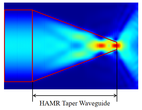
The HAMR tapered waveguide is integrated into the magnetic recording write head. Its width gradually decreases along the propagation direction, compressing the wide mode field input from the laser, so that the optical field is stably confined near the waveguide center, improving the stability of optical energy transmission and alignment tolerance. It is a key component for achieving nanoscale spot focusing. Based on reference [1], this example builds two similar HAMR simulation models: the first uses a higher-index substrate and a Gaussian source, and performs broadband simulation with the 2.5D finite-difference time-domain (FDTD) solver; the second uses a uniform cladding around the waveguide core and performs single-frequency simulation with the eigenmode expansion (EME) solver and the 2.5D FDTD solver. By comparing the applicable conditions of the two models, this example provides a basis for selecting a simulation approach for HAMR tapered waveguides.
Simulation Settings
Structure Model
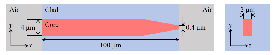
The HAMR tapered waveguide simulated in this example is shown in the figure below. The waveguide core material is , with a total length of . Within the long taper region, the waveguide width gradually transitions from to , achieving compression of the optical field from the micrometer to the nanoscale.
To compare the advantages of different solvers and sources, this example builds two models with similar structures but different cladding and substrate settings. The main differences are shown in the table below.
| Parameter | Broadband Gaussian Source Model | Single-Frequency Mode Source Model |
|---|---|---|
| Cladding/Substrate | substrate, air above the core | cladding around the core |
| Source | Gaussian source | Mode source |
| Wavelength | ||
| Solver | 2.5D FDTD | EME / 2.5D FDTD |
In the broadband Gaussian source model, the device uses an substrate with air above the core. A focused Gaussian beam is coupled from air into the waveguide along the positive direction, with an incident wavelength range of . In the single-frequency mode source model, the source wavelength is , the waveguide geometry is unchanged, but is used to clad the core.
Simulation Results
Broadband 2.5D FDTD Simulation Results
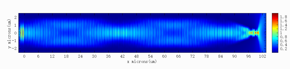
The HAMR_taper_waveguide_Gaussian.mpps project in the attachment is a broadband simulation model based on the 2.5D FDTD solver. This model aims to obtain the broadband response and to simulate light propagation in the air region after the taper output end. The figure below shows the electric field result in the waveguide at a wavelength of . It can be seen that after the incident light is coupled from air into the waveguide, the optical field is mainly confined in the wide waveguide core; as the waveguide width gradually decreases to within the taper region, the optical field is progressively compressed to the submicron scale.
For this model, the 2.5D FDTD solver has the following advantages:
- The 2.5D FDTD solver reduces the 3D structure to a 2D simulation based on the effective index method, significantly improving simulation speed while maintaining calculation accuracy;
- A broadband simulation result can be obtained in a single simulation, without the need to run the simulation frequency by frequency over a wide range as with EME, resulting in higher efficiency;
- In the region after the taper output end, the cross-section of the EME solver contains air and the substrate below, with no high-index core. The modes calculated in this case are mainly modes confined in the substrate, while modes that overlap with the taper output field and propagate in the air region account for only a small portion. Therefore, the EME solver needs to solve a large number of modes to accurately describe the field distribution in this region; in contrast, the 2.5D FDTD solver can directly simulate this region without solving a large number of modes.
Single-Frequency EME / 2.5D FDTD Simulation Results
EME Mode Convergence Verification
The HAMR_taper_waveguide_Mode.mpps project in the attachment is a single-frequency simulation model that uses both the EME and 2.5D FDTD solvers. The EME solver divides the device into a number of cells along the propagation direction, solves a certain number of eigenmodes in each cell, and calculates the reflection and transmission coefficients between cells through mode expansion. In practice, the number of modes is finite, and the results vary with the number of modes, so mode convergence must be verified.
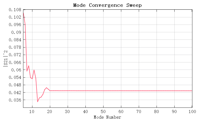
First, a mode convergence sweep is performed. Run the HAMR_taper_waveguide_Mode_convergence.msf script. The script sets the starting mode number for the mode convergence sweep to with an interval of . After the sweep, the curve of versus the number of modes is obtained, as shown in the figure below. When the number of modes is less than , fluctuates drastically as the number of modes increases; when the number of modes reaches about , the curve becomes flat, and further increasing the number of modes has almost no effect on the result. This indicates that for the S-parameters, about modes are sufficient.
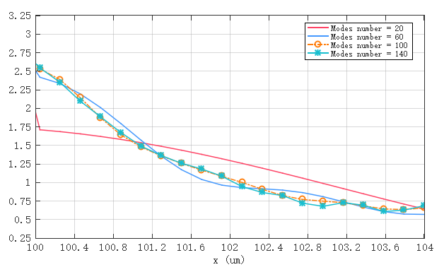
However, the S-parameters mainly reflect the energy transmission characteristics of the waveguide and the taper region, and do not fully represent the convergence of the field distribution in the air region after the taper output end. This is because light diverges and propagates in different directions in the air region after exiting the taper end, requiring a large number of modes to accurately represent the field distribution in that region. To determine the number of modes required for convergence in the air region, the number of modes in the air region is varied, and the electric field amplitude along the direction at is extracted. The results are shown in the figure below. When the number of modes in the air region reaches about , the differences between the curves for different mode numbers are significantly reduced; further increasing the number of modes to above makes the results stabilize, indicating that the field distribution in the air region has basically converged. Therefore, in the EME solver, the number of modes in the air region after the taper output end is set to .
EME / 2.5D FDTD Field Distribution
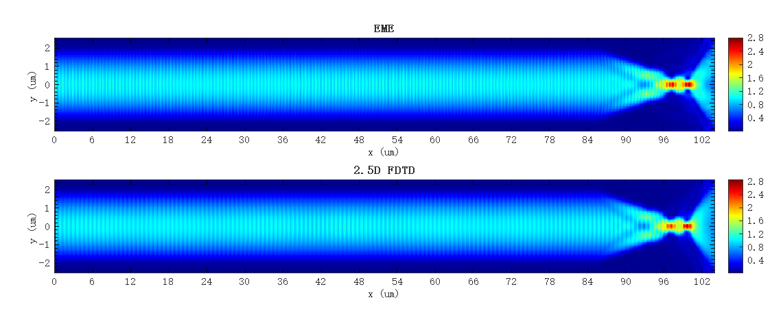
Run the HAMR_taper_waveguide_Mode.msf script. The script performs simulations using the EME and 2.5D FDTD solvers separately and plots the results. The 2D electric field simulation results of the two solvers are shown below. It can be seen that the electric field distributions obtained by the two solvers are highly consistent.
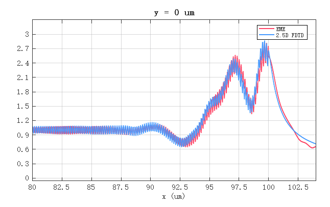
To more precisely compare the results of the two solvers, the electric field amplitude along the direction at is extracted, as shown in the figure below. The curves of EME and 2.5D FDTD are essentially consistent throughout the propagation process, showing good agreement between the two solvers in the single-frequency mode source simulation. The EME solver can simultaneously complete mode solving and S-parameter extraction in a single run, with a computation speed far faster than the 2.5D FDTD solver, demonstrating a clear speed advantage in such single-frequency simulations with both reliability and efficiency.
For this model, the EME solver has the following advantages:
- If the waveguide or taper region length needs to be optimized, after the simulation run, the propagation sweep function in the EME analysis window can quickly obtain simulation results for different lengths without re-running the simulation; in contrast, the 2.5D FDTD solver requires a separate simulation run for each length, affecting simulation and optimization efficiency;
- The EME solver can obtain the results of multiple modes simultaneously in a single simulation and extract the S-parameters of all modes; the 2.5D FDTD solver requires injecting individual modes separately and re-running the simulation, resulting in lower efficiency.
In summary, the two solvers each have their own advantages, and the choice should be made on a case-by-case basis. The EME solver is more advantageous for parameter sweeps of long waveguide structures and S-parameter extraction, making it an efficient tool for waveguide design and optimization; the 2.5D FDTD solver is more suitable for simulation scenarios requiring broadband response, strong radiation fields or free propagation in air, abrupt cross-section changes, or strong loss.
References
[1] K. Takano, et al., "Optical Design Challenges of Thermally Assisted Magnetic Recording Heads," IEEE Trans. Magn., 46(3), 744-750 (2010).