Finite Difference Eigenmode Solver (FDE)
SimWorks FDE is a powerful tool for researchers and engineers to solve problems of large-scale integrated planar optical waveguides, long-distance transmission devices, and various new types of optical fibers. We will briefly introduce the physical principles and key features.
Basic Principles of the FDE Solver
Finite Difference Eigenmode (FDE) Solver calculates the spatial distributions and frequency characteristics of eigenmodes by solving Maxwell's equations on a cross-sectional mesh of waveguide-like structures. The basic principles of FDE are outlined as follows.
By adjusting the coefficients of frequency domain Maxwell's curl equation, it can be simplified to the following form:
According to the general form of the mode in the waveguide, the electric and magnetic fields can be written as and , which can be substituted into Maxwell's curl equation to obtain the expression of electromagnetic field component. For example, z-axis magnetic field component:
When linear expansion is done along the coordinate axis in space, the above equation can be transformed into the following matrix form:
The six matrix equations of the electromagnetic field components can be converted into the problem of solving the eigenvalues:
The matrix represents the coefficient matrix of the difference algorithm, the vector represents the electromagnetic field components to be solved, and the represents the propagation constant.
After 2D 'Yee cell' mesh is generated on the cross section of the waveguide structure, the material parameters, electric field and magnetic field can be reflected at each mesh point. In this algorithm, the sparse matrix technique is used to solve eigenvalue of the matrix, which generates the corresponding mode distribution and effective refractive index.
-
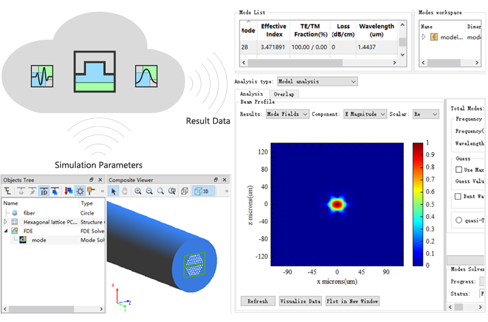
Mode Data
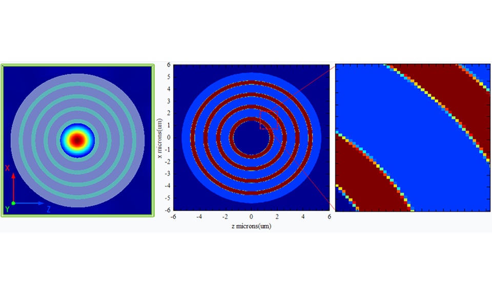
When the FDE solver type is selected as 2D Y normal, the simulation results are shown below.
- The spatial distribution of the Y-axis vector field
-
Effective Index
Calculate the effective index of the mode using the following formula:
Where is the angular frequency, is the propagation constant of the mode, is the speed of light in vacuum, is group velocity of the mode, and is the wave vector in free space .
-
TE/TM fraction
TE/TM fraction (TE/TM fraction (%)) describes the polarization properties of a mode on the cross‑section. For a mode propagating along the z direction, the TE polarization fraction is defined by the component, and its calculation formula is:
Here, and are the two orthogonal electric‑field components perpendicular to the propagation direction, and is the integration area on the mode cross‑section. When the propagation direction is along the x axis, the TE polarization fraction is defined by ; for other propagation directions, the definition follows the same principle.
-
Loss
The transmission Loss (Loss(dB/cm)) of the mode is calculated as:
Wherein, is the imaginary part of the complex refractive index.

Basic Principles of the Mode Coupling Algorithm
Mode coupling is used to calculate the field overlap and coupling efficiency between one input mode in one waveguide and all modes in the other waveguide. The basic principle of the mode coupling algorithm is outlined as follows.
For an interface input field , and output field , , the input and output power are respectively:
Since any field in a waveguide can be viewed as a combination of a basis consisting of a sequence of orthogonal modes, in the case of negligible reflection fields, the input and output fields can be expressed as follows:
The coefficients and are calculated by the following formulas:
The total power of the transmitted output field can thus be calculated as follows:
The mode coupling coefficient of the ith mode is calculated as follows:
The result of mode coupling shows how much power the field of the ith mode can be carried in a given input field. It should be noted that this algorithm is calculated based on the ideal case, and the calculation results may not be accurate when there is reflection or waveguide loss during transmission. For a detailed introduction, see Snyder and Love's "Optical Waveguide Theory".
Key Features of the FDE Solver
3D CAD interface and rich structure library
- The Multi-view 3D CAD platform helps model construction.
- The built-in rich waveguide structure library can quickly build a variety of the waveguide structures.
- Allow direct import of GDS files to adjust the complicated structures.

Mesh technology
- Support auto non-uniform mesh and custom mesh to improve the efficiency of 2D Yee cell mesh construction for complex waveguide structure sections.
- Support the advanced techniques of conformal mesh to get more accurate results, including: Volume-average polarized effective permittivity (VPEP), Volume average (VEP), Yu-Mittra 1, Yu-Mittra 2.
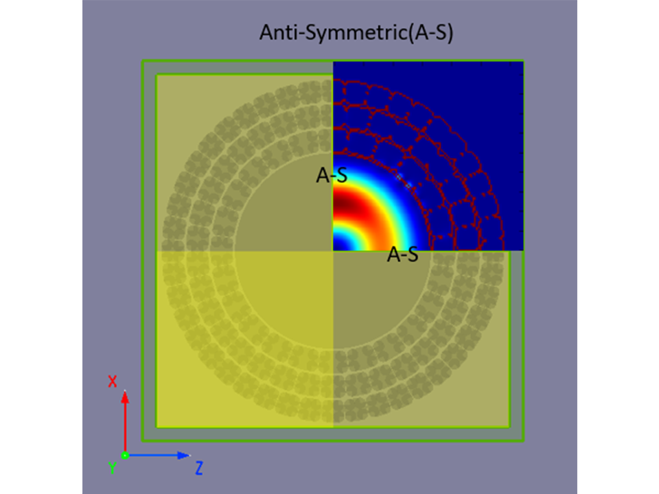
Boundary conditions
- Offer various boundary conditions, for example, perfectly-matched layer (PML), periodic, Bloch, symmetric or anti-symmetric, perfect electrical conductor (PEC) or perfect magnetic conductor (PMC).
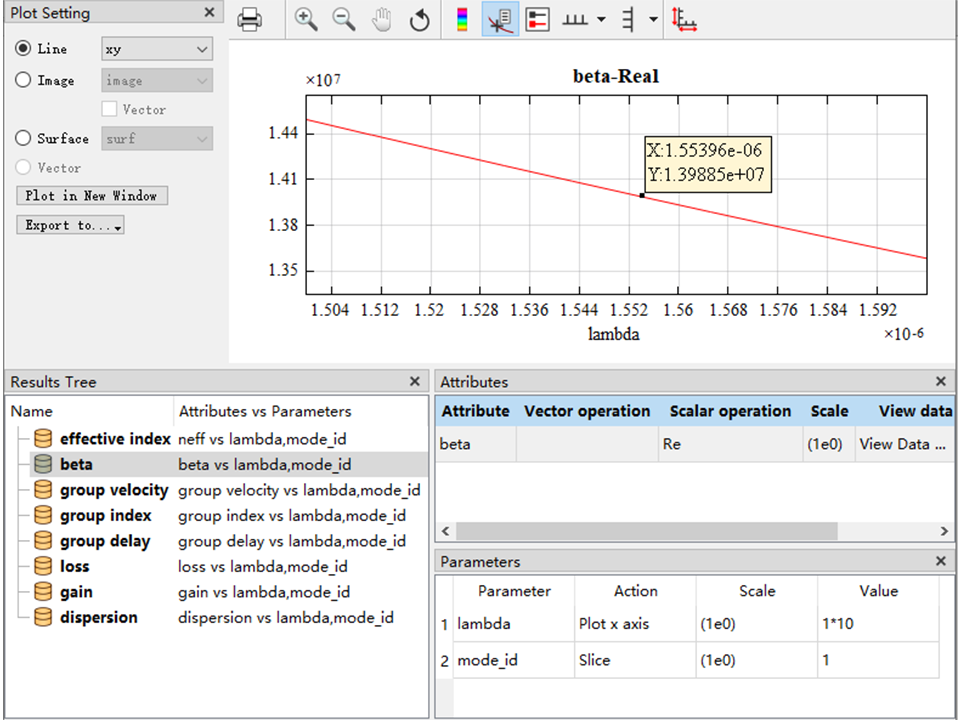
Frequency analysis
- Data visualization and frequency analysis can be performed for all the modes of the structure.
- The feature of mode coupling allows users to analyze mode overlap and calculate the coupling efficiency between different modes.
- Support frequency sweep to quickly obtain key data such as mode group velocity, loss, and dispersion.
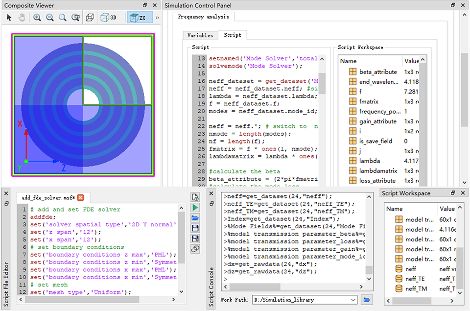
Script control
- Enable users to control each steps in the simulation by scripts to perform the parametric operations.
- The complete function libraries basically meet all the needs of mathematical calculations, and the custom functions are allowed too.
Computing power
- The computing power and mode solution speed are improved dramatically with the help of OpenMP, MPI, AVX and other parallel computing technologies.
- Provide cloud-based mode solution services, so users are no longer limited to the local computing resources.
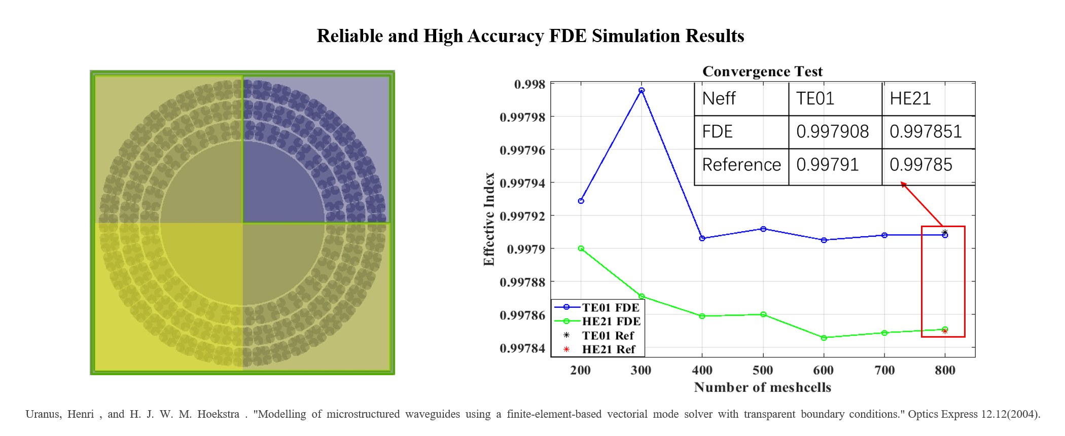
Ultra-high computational accuracy
- The FDE algorithm uses mode coupling to model optical waveguides and can achieve highly accurate modeling results. For example, in the mode solution of hollow photonic crystal fibers, it is highly sensitive to small variations in the mesh size. After convergence tests, the relative error between SimWorks' results and the literature is only 0.0001%, demonstrating the ultra-high computational accuracy of the SimWorks' FDE algorithm.
Application Examples
References
[1]Zhaoming Zhu and Thomas G. Brown, "Full-vectorial finite-difference analysis of microstructured optical fibers," Opt. Express 10, 853-864 (2002)