SimWorks Stack Solver (STACK)

SimWorks Stack Solver (STACK) analyzes thin-film structures composed of parallel, homogeneous layers. Electromagnetic waves propagate through the layers and undergo reflection and transmission at their interfaces, producing multiple reflections and interference. Using the refractive indices, layer thicknesses, and continuity conditions for electromagnetic fields, STACK determines both the response to incident plane waves and the emission characteristics of embedded dipoles without spatial meshing of the entire structure.

(1) Reflection and Transmission (stackrt)

For an incident plane wave, the reflectance and transmittance of a multilayer stack depend on the refractive indices, layer thicknesses, and incidence angle, as illustrated in Figure 1.

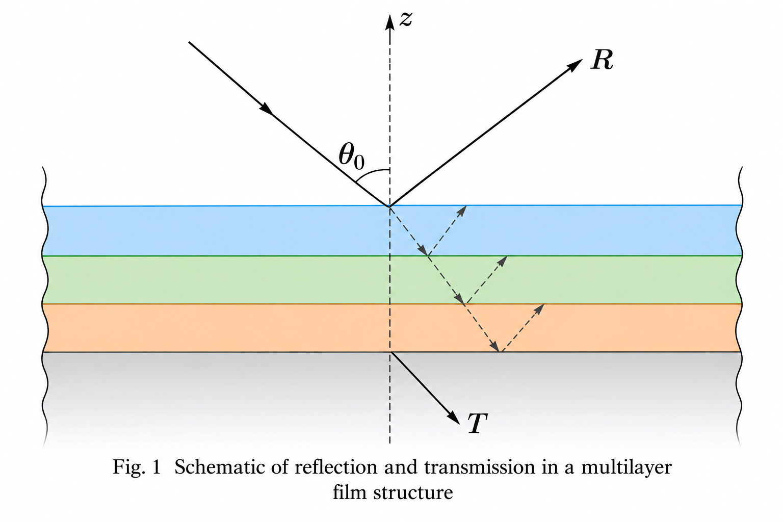
The $z$ axis in Figure 1 indicates the interface normal, $\theta_0$ is the incidence angle, and $R$ and $T$ are reflectance and transmittance. The refractive indices of the incident and exit media are $n_0$ and $n_s$, while $n_j$ and $d_j$ denote the refractive index and thickness of layer $j$. For lossless isotropic media, adjacent layers satisfy $n_j\sin\theta_j=n_{j+1}\sin\theta_{j+1}$.

STACK uses the transfer matrix method (TMM) to describe propagation and interference in the multilayer structure. For an isotropic, lossless, nonmagnetic film, the phase accumulated in layer $j$ is

$$\delta_j=\frac{2\pi}{\lambda}n_jd_j\cos\theta_j$$

where $\lambda$ is the vacuum wavelength and $\theta_j$ is the propagation angle in layer $j$. Forward- and backward-propagating waves acquire phase factors $e^{\pm i\delta_j}$. Together with the continuity of tangential electric and magnetic fields at interfaces, this gives the characteristic matrix of layer $j$:

$$M_j=\begin{pmatrix} \cos\delta_j & -\dfrac{i\sin\delta_j}{Y_j}\\[6pt] -iY_j\sin\delta_j & \cos\delta_j \end{pmatrix}$$

Here $i$ is the imaginary unit, and $Y_j$ is the optical admittance. For s and p polarization, respectively,

$$Y_j^{(s)}=\frac{n_j\cos\theta_j}{Z_0},\qquad Y_j^{(p)}=\frac{n_j}{Z_0\cos\theta_j}$$

where $Z_0$ is the vacuum impedance. The phase terms describe propagation within the layer, while the admittance relates the tangential electric and magnetic fields for each polarization.

For $N$ finite-thickness layers, the characteristic matrices are multiplied in layer order to obtain the total matrix:

$$M_{\mathrm{stack}}=M_1M_2\cdots M_N$$

The total characteristic matrix connects the tangential electric and magnetic fields at the incident and exit sides of the multilayer stack. The incident-side fields combine incident and reflected waves; when no wave is incident from the exit side, only the transmitted wave remains there. Together with the optical admittances and boundary conditions of the outer media, this relation gives the complex reflection and transmission amplitude coefficients $r$ and $t$.

Reflectance and transmittance are power ratios, not amplitude ratios. The Poynting vector of the electric and magnetic fields gives the time-averaged power flux normal to the interfaces, allowing the amplitude coefficients to be converted into reflectance and transmittance. For a given s or p polarization in isotropic materials with lossless incident and exit media,

$$R=\frac{P_{\mathrm{ref}}}{P_{\mathrm{inc}}},\qquad T=\frac{P_{\mathrm{trans}}}{P_{\mathrm{inc}}}$$

where $P_{\mathrm{inc}}$, $P_{\mathrm{ref}}$, and $P_{\mathrm{trans}}$ denote the magnitudes of incident, reflected, and transmitted power fluxes normal to the interfaces. For anisotropic materials, the energy-flow properties of different modes require corresponding power normalization.

(2) Internal Electromagnetic Fields (stackfield)

Reflectance and transmittance describe the overall optical response of the multilayer stack, while the internal electromagnetic fields also depend on the superposition of forward- and backward-propagating waves. For a finite-thickness, isotropic, lossless layer, the normal wave-vector component in layer $j$ is first determined from the refractive indices and angle of incidence:

$$k_{z,j}=k_0n_j\cos\theta_j =\frac{2\pi}{\lambda}\sqrt{n_j^2-n_0^2\sin^2\theta_0}, \qquad k_0=\frac{2\pi}{\lambda}$$

After obtaining the overall reflection and transmission amplitudes using the transfer matrix method, the characteristic matrices yield the tangential electric and magnetic fields at the layer interfaces. Taking the incident-side interface of layer $j$ as the reference gives

$$\begin{pmatrix} E_{t,j}\\ H_{t,j} \end{pmatrix} = M_jM_{j+1}\cdots M_N \begin{pmatrix} tE_{\mathrm{inc}}\\ Y_stE_{\mathrm{inc}} \end{pmatrix}$$

where $E_{t,j}$ and $H_{t,j}$ are the tangential electric and magnetic fields at that interface, $E_{\mathrm{inc}}$ is the incident tangential electric-field phasor, and $t$ is the transmission amplitude coefficient defined for tangential electric fields; thus $tE_{\mathrm{inc}}$ is the transmitted tangential electric field. The exit-medium optical admittance is $Y_s$. For p polarization, this $t$ differs from the transmission coefficient defined using the total electric-field amplitude.

The complex amplitudes of the forward- and backward-propagating waves follow from the superposition of the tangential electric and magnetic fields at the interface:

$$E_j^+=\frac12\left(E_{t,j}+\frac{H_{t,j}}{Y_j}\right), \qquad E_j^-=\frac12\left(E_{t,j}-\frac{H_{t,j}}{Y_j}\right)$$

Here $E_j^+$ and $E_j^-$ are the complex amplitudes of the forward- and backward-propagating waves in layer $j$, respectively, and $Y_j$ is the optical admittance for the corresponding polarization in that layer.

Combining these amplitudes with the propagation phase gives the tangential complex electric field at local coordinate $z$ in layer $j$ (measured from its incident-side interface toward the exit side):

$$E_j(z)=E_j^+e^{ik_{z,j}z}+E_j^-e^{-ik_{z,j}z}$$

For absorbing or anisotropic media, the normal wave-vector component and field relations depend on the material parameters and polarization state. This procedure yields the internal electromagnetic-field distribution for analyzing thin-film interference and local field enhancement.

(3) Purcell Factor (stackpurcell)

The preceding sections consider light incident from outside the structure. In light-emitting devices such as OLEDs, the source may instead be an electric dipole embedded within one of the film layers. The emitted waves travel in different directions and undergo reflection and transmission at surrounding interfaces. Fields returning toward the dipole modify the total power it delivers to the electromagnetic field, while outgoing waves form a directional radiation pattern. Figure 2 illustrates these two effects in the same physical setting.

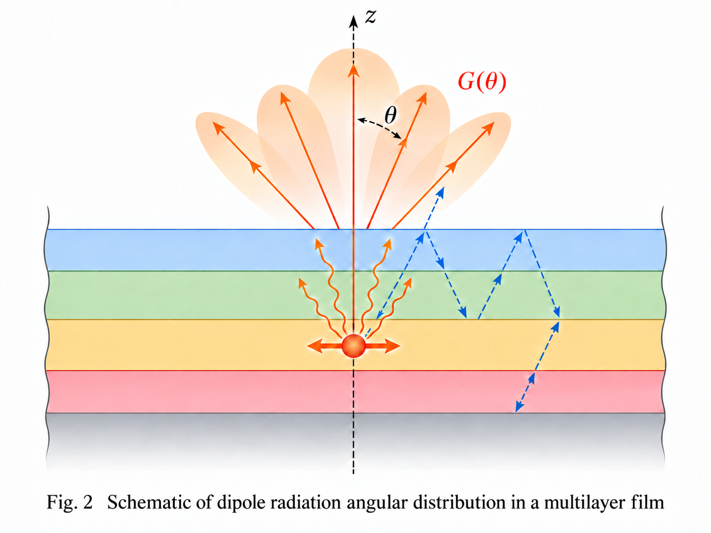
In Figure 2, different colors distinguish the thin-film layers. The orange dot represents an electric dipole embedded in one existing host layer, not an additional layer. Orange arrows and the upper angular pattern illustrate outward emission; blue dashed arrows schematically indicate feedback from multiple interface reflections. The $z$ axis points upward, $\theta$ is the emission angle relative to the upward surface normal, and $G(\theta)$ denotes the angle-dependent emission result. The host-layer index is denoted by $n_h$, and the upper and lower outer-medium indices by $n_0$ and $n_s$ in the accompanying equations; these symbols are not individually labeled in the illustration. The combined reflected field can modify the dipole's total emitted power, while outward waves determine its far-field angular distribution. The arrows illustrate these effects qualitatively and do not encode exact refraction angles at every interface.

For a dipole in a lossless host layer, the Purcell factor is defined as the ratio of its total power delivered in the multilayer structure to the corresponding power in an infinite homogeneous reference medium:

$$F_{\mathrm P}(\lambda)= \frac{P_{\mathrm{stack}}(\lambda)}{P_{\mathrm{hom}}(\lambda)}$$

Here $F_{\mathrm P}$ is the Purcell factor, $P_{\mathrm{stack}}$ is the total power delivered by the dipole to the electromagnetic field in the multilayer structure, $P_{\mathrm{hom}}$ is the reference power for the same dipole in an infinite homogeneous medium matching its host layer, and $\lambda$ is the emission wavelength. Values $F_{\mathrm P}>1$ and $F_{\mathrm P}<1$ indicate enhancement and suppression of total power relative to that reference.

The Purcell factor describes total power, not directly the far-field power extracted from the device. In absorbing structures, some energy may also be dissipated non-radiatively. The related calculations can additionally evaluate upward, downward, and into-air angular far-field power densities.

(4) Dipole Emission (stackdipole)

For multilayer light-emitting devices, in addition to changes in the dipole's total power, its angular emission characteristics must be analyzed together with the emission spectrum. STACK spectrally weights the far-field angular power density by accounting for the dipole position, orientation, emission spectrum, and emission-efficiency parameters.

For multiple dipoles with continuous emission spectra, the spectrum-weighted angular emission can be expressed as

$$G(\theta)=\sum_m \int_{\lambda_{\min}}^{\lambda_{\max}} \frac{ef_m\,st_m\,rd_m\,p_m(\lambda)\,E_\gamma(\lambda)\, f_{\mathrm{rad},m}(\theta,\lambda)} {rd_m F_{\mathrm P,m}(\lambda)+(1-rd_m)}\,d\lambda$$

where $G(\theta)$ is the spectrum-weighted angular emission result for the selected exit side at angle $\theta$; $\theta$ is measured in that side's outermost medium from the outward normal and does not necessarily denote an angle in air; $m$ indexes dipoles; $\lambda_{\min}$ and $\lambda_{\max}$ define the wavelength range; $ef_m$, $st_m$, and $rd_m$ are the exciton formation fraction, singlet-exciton fraction, and relative radiative decay fraction; $f_{\mathrm{rad},m}(\theta,\lambda)$ is the far-field angular power density per unit solid angle, normalized to the total power of the same dipole in the infinite homogeneous host medium; and $F_{\mathrm P,m}(\lambda)$ is the corresponding Purcell factor.

The photon energy in electronvolts (eV) is numerically given by

$$E_\gamma(\lambda)=\frac{hc}{e\lambda}$$

where $h$ is Planck's constant, $c$ is the speed of light in vacuum, and $e$ is the magnitude of the elementary charge. The quantity $p_m(\lambda)$ is the wavelength-normalized photon emission probability density and satisfies

$$\int_{\lambda_{\min}}^{\lambda_{\max}}p_m(\lambda)\,d\lambda=1$$

For an input emission spectrum $S_m(\lambda)$, the continuous spectral weight can be written as

$$p_m(\lambda)= \frac{S_m(\lambda)/f(\lambda)} {\displaystyle\int_{\lambda_{\min}}^{\lambda_{\max}}S_m(\lambda')/f(\lambda')\,d\lambda'}, \qquad f(\lambda)=\frac{c}{\lambda}$$

where $f(\lambda)$ is the optical frequency and $\lambda'$ is a dummy integration variable. The integral describes how all wavelengths contribute to angular emission in the continuous model; numerical implementations use discrete wavelength samples. $G(\theta)$ is a model-scaled, spectrum-weighted result rather than absolutely calibrated radiance. CIE 1931 color-matching functions can also be used to analyze luminance-related quantities and tristimulus values.

This provides a combined analysis of the spectral and angular characteristics of multilayer light-emitting devices.

References

[1] P. Yeh, Optical Waves in Layered Media, Wiley, 1988.
[2] K. A. Neyts, "Simulation of light emission from thin-film microcavities," Journal of the Optical Society of America A, vol. 15, no. 4, 1998.
[3] W. Lukosz and R. E. Kunz, "Light emission by magnetic and electric dipoles close to a plane interface," Journal of the Optical Society of America, vol. 67, pp. 1607–1619, 1977.