Preface #

With the rapid development of artificial intelligence and machine learning technologies, data centers are placing higher demands on the bandwidth, energy efficiency, and integration level of interconnect architectures. Photonic integrated circuits (PICs) and co-packaged optics (CPO) solutions have become core technologies for breaking through traditional interconnect bottlenecks. However, as the industry advances toward 3D stacking and high integration, the design of interlayer coupling for optical signals directly affects packaging complexity, technical cost, and manufacturing yield. In such multilayer vertical integration schemes, because the active and passive waveguides are closely stacked in the vertical direction and differ in material refractive index and mode field distribution, direct butt coupling leads to severe mode mismatch and coupling loss.

To efficiently transfer light from the passive waveguide to the active waveguide, a vertical coupler can be used, which is a key device for vertical transmission of optical signals. By gradually narrowing the passive waveguide from a wide section to a tip while gradually widening the active waveguide from a narrow tip to a wide section, the vertical coupler enables light to be adiabatically transferred from one layer to another within the taper region, offering the advantages of low loss and high tolerance. To maintain high coupling efficiency while reducing the size of the vertical coupler, two key parameters need to be optimized: first, the lateral offset (misalignment) of the active waveguide tip relative to the passive waveguide, to minimize mode mismatch at the entrance; second, the length of the taper region (taper length), to balance adiabatic evolution and transmission loss.

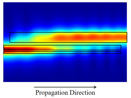
Based on reference [1], this example designs and simulates a vertical coupler for a dual-layer integrated platform of $\mathrm{Si_3N_4}$ and $\mathrm{Al_2O_3:Er^{3+}}$ (abbreviated as $\mathrm{Al_2O_3}$ hereinafter). First, the finite-difference eigenmode (FDE) solver is used to analyze the mode overlap between the $\mathrm{Si_3N_4}$ and $\mathrm{Al_2O_3}$ waveguides and determine the optimal lateral offset; then, the eigenmode expansion (EME) solver is used to sweep the taper region length to optimize the coupling efficiency; finally, the finite-difference time-domain (FDTD) solver is used for verification. The simulation results show that the coupling efficiency is better than $\mathrm{-0.3\ dB}$ over the wavelength range of $\mathrm{1480–1620\ nm}$ .

Simulation Settings #

Structure Model #

The schematic of the vertical coupler simulated in this example is shown below. The device consists of a $\mathrm{Si_3N_4}$ waveguide, an $\mathrm{Al_2O_3}$ waveguide, a $\mathrm{SiO_2}$ spacer layer, and a cladding. The $\mathrm{Si_3N_4}$ waveguide has a thickness of $\mathrm{350\ nm}$ and adopts a TriPleX asymmetric double stripe (ADS) structure, which is divided into two parts by a $\mathrm{100\ nm}$ thick $\mathrm{SiO_2}$ spacer layer in the middle; the $\mathrm{Al_2O_3}$ waveguide is located $350\ \mathrm{nm}$ above the $\mathrm{Si_3N_4}$ waveguide and has a thickness of $\mathrm{750\ nm}$ . Considering that the sidewalls cannot be perfectly vertical in practical etching processes, the sidewall angle of both waveguides is set to $10^\circ$ in the simulation.

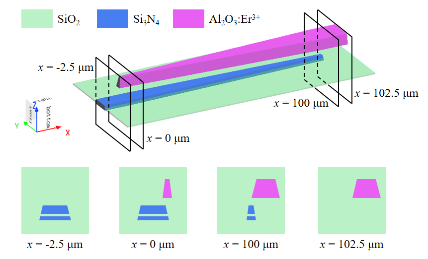
The $\mathrm{Si_3N_4}$ material uses the Si3N4 (Silicon Nitride) - Luke model, and the $\mathrm{SiO_2}$ material uses the SiO2 (Glass) - Palik model; since the refractive index of $\mathrm{Al_2O_3}$ changes very little over the operating wavelength band and the influence of $\mathrm{Er}$ doping on the refractive index is negligible, $\mathrm{Al_2O_3}$ is set as a Dielectric material with $\mathrm{n=1.724}$ in the simulation. In addition, the background material of the simulation region is set to the SiO2 (Glass) - Palik model to simulate the actual operating environment of the device.

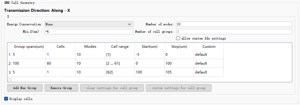
In terms of solver settings, to sweep the length of the taper region, the EME solver is divided into three cell groups along the propagation direction (X direction), as shown in the figure below. Cell group 2 is the taper region, where 60 cells are set to accurately resolve the gradual variation of the geometry along the propagation direction. Ten modes are solved in each cell group to fully capture the mode evolution within the taper region.

Simulation Results #

FDE-Based Mode Overlap Analysis #

Along the propagation direction, the vertical coupler can be divided into three parts: the $\mathrm{Si_3N_4}$ waveguide region, the composite structure region formed by the overlap of two tapered waveguides, and the $\mathrm{Al_2O_3}$ waveguide region. The total loss of the vertical coupler mainly consists of three parts: the mode mismatch between the $\mathrm{Si_3N_4}$ waveguide and the composite structure at the entrance (where the $\mathrm{Al_2O_3}$ waveguide begins to appear), the mode mismatch between the composite structure and the $\mathrm{Al_2O_3}$ waveguide at the exit (where the $\mathrm{Si_3N_4}$ waveguide ends), and the mode evolution loss within the taper region. In this example, the FDE solver is first used to analyze the mode overlap at the entrance to determine the optimal lateral offset.

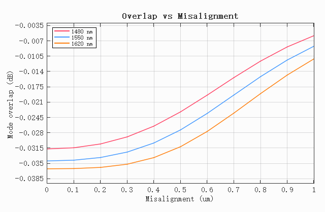
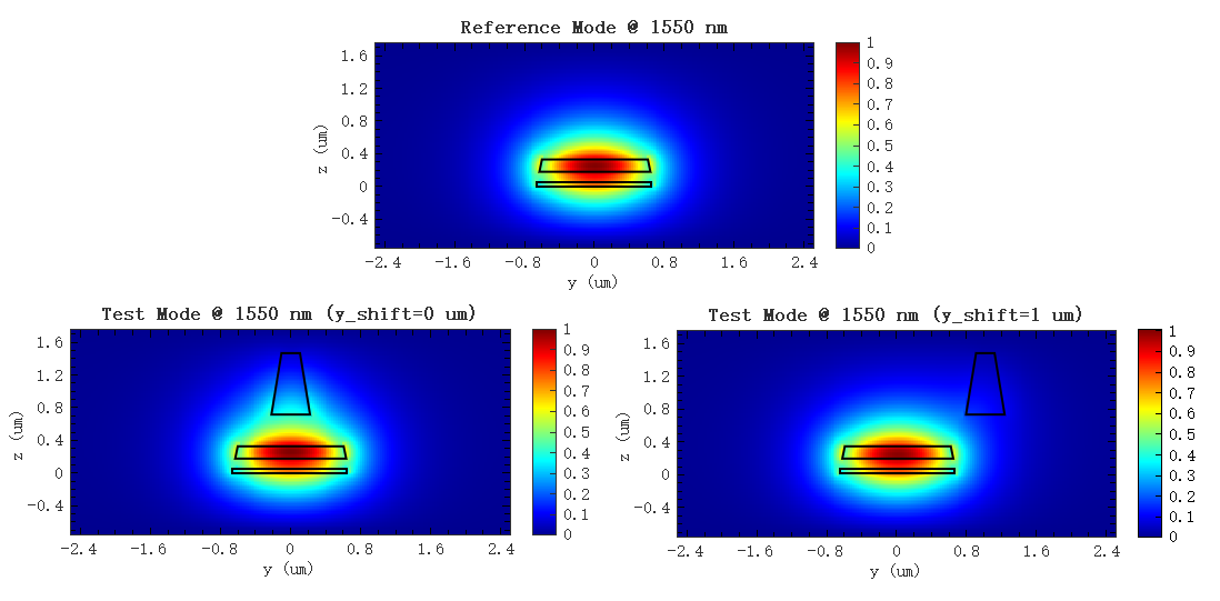
Open the attached vertical_coupler_FDE.mpps project and run the vertical_coupler_FDE.msf script. The script solves the fundamental mode of the $\mathrm{Si_3N_4}$ waveguide at $x = -2.5\ \mathrm{μm}$ as the reference mode, and then solves the mode of the composite structure formed by the $\mathrm{Si_3N_4}$ waveguide and the $\mathrm{Al_2O_3}$ waveguide at $x = 0\ \mathrm{μm}$ as the test mode. These two cross-sections correspond to $\mathrm{CS_1}$ and $\mathrm{CS_2}$ in the paper, respectively. Subsequently, a lateral offset is applied to the $\mathrm{Al_2O_3}$ waveguide over the range of $0$ to $1\ \mathrm{μm}$ , and the mode mismatch between the test mode and the reference mode is calculated at each offset for different wavelengths. The simulation results are shown below. It can be seen that the mode mismatch is largest at an offset of $0$ , and the mismatch becomes more severe at longer wavelengths, with the mismatch at $\mathrm{1620\ nm}$ reaching $-0.036\ \mathrm{dB}$ ; as the offset increases, the mode mismatch at all three wavelengths gradually decreases, with a consistent trend. When the offset reaches $1\ \mathrm{μm}$ , the mode mismatch drops to about $-0.011\ \mathrm{dB}$ , which is consistent with the conclusion in the paper.

To more intuitively compare the influence of different lateral offsets on mode mismatch, the figure below shows the mode field distributions of the reference mode and the test modes at two offsets at $1550\ \mathrm{nm}$ . It can be seen from the figure that when the offset is $0$ , the $\mathrm{Al_2O_3}$ waveguide is located directly above the $\mathrm{Si_3N_4}$ waveguide, the field distribution is perturbed, and it differs significantly from the reference mode; when the offset is $1\ \mathrm{μm}$ , the $\mathrm{Al_2O_3}$ waveguide is moved to the edge of the $\mathrm{Si_3N_4}$ waveguide, its influence on the fundamental mode is weakened, and the field distribution is closer to the reference mode. Therefore, the lateral offset of the $\mathrm{Al_2O_3}$ waveguide is set to $1\ \mathrm{μm}$ in the subsequent simulation.

EME-Based Taper Region Length Sweep #

The length of the taper region determines whether the mode can maintain adiabatic evolution during the gradual transition: if the length is too short, non-adiabatic coupling occurs, and part of the energy is transferred to higher-order modes or radiation modes, causing additional loss; when the length increases to a certain extent, the mode evolution is already close to adiabatic, and further increasing the length provides very limited improvement in coupling efficiency while increasing the device size. Therefore, after determining the optimal lateral offset, this example uses the EME solver to sweep the taper region length to analyze the mode evolution loss within the taper region of the vertical coupler and determine the optimal value that balances coupling efficiency and device size.

Run the vertical_coupler_EME.msf script in the vertical_coupler_EME.mpps project. The script sweeps the taper region length at different wavelengths and calculates the power transmission coefficient $|S_{21}|^2$ . During the sweep, the taper region length varies from $100\ \mathrm{μm}$ to $1000\ \mathrm{μm}$ , and the results are shown below. When the taper length is short, the power transmission loss is relatively large; as the length increases, the loss decreases rapidly and tends to saturate after about $400\ \mathrm{μm}$ , reaching about $-0.029\ \mathrm{dB}$ , which is basically consistent with the results in the paper. The curves at the three wavelengths have the same trend, and after the length reaches $400\ \mathrm{μm}$ , the difference in power transmission among the three wavelengths is small, indicating good broadband characteristics.

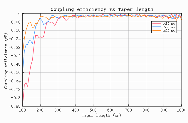
Due to practical design considerations, the paper sets the taper region length to $800\ \mathrm{μm}$ . However, considering the subsequent FDTD simulation, further increasing the taper region length results in little change in coupling efficiency. Instead, as the device size increases, the simulation speed significantly decreases. Therefore, this example adopts $400\ \mathrm{μm}$ as the taper region length.

FDTD-Based Verification #

To verify the performance of the vertical coupler in an actual three-dimensional structure, this example uses the FDTD solver for simulation, employing a Port Group as the mode light source and monitor, exciting the fundamental mode at the $\mathrm{Si_3N_4}$ input end and extracting the output power at the $\mathrm{Al_2O_3}$ output end. The taper region length is set to $400\ \mathrm{μm}$ , and the lateral offset is set to $1\ \mathrm{μm}$ . Run the vertical_coupler_FDTD.msf script in the vertical_coupler_FDTD.mpps project. After the simulation, the script extracts the power transmission coefficient $|S_{21}|^2$ at three wavelengths, and the results are shown below.

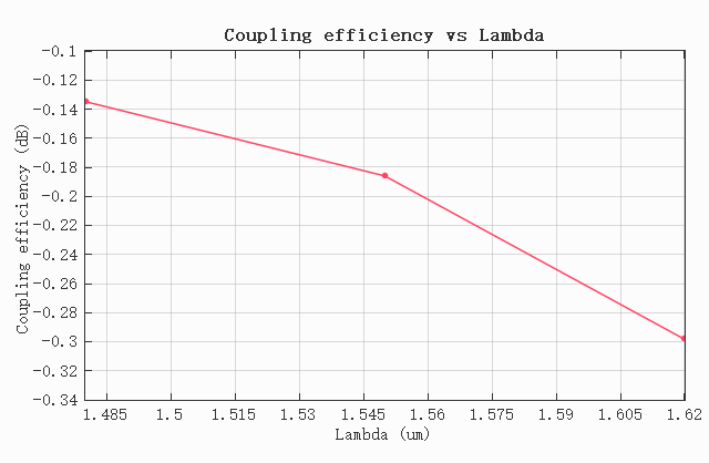
It can be seen from the figure that the coupling efficiency is about $-0.14\ \mathrm{dB}$ at $1480\ \mathrm{nm}$ , about $-0.19\ \mathrm{dB}$ at $1550\ \mathrm{nm}$ , and about $-0.30\ \mathrm{dB}$ at $1620\ \mathrm{nm}$ . The FDTD results are slightly lower than the EME results, but the trends are consistent, and the coupling efficiency at all three wavelengths is better than $-0.3\ \mathrm{dB}$ , verifying the reliability of the design. In addition, the longer the wavelength, the weaker the mode confinement, and the coupling efficiency decreases slightly, which is also consistent with the trend observed in the mode overlap analysis. The above results show that the simulated vertical coupler has low-loss, broadband mode conversion characteristics over the wavelength range of $\mathrm{1480–1620\ nm}$ .

References #

[1] C. E. Osornio-Martinez, et al., "Monolithically integrated erbium-doped polycrystalline Al₂O₃ waveguide amplifier on silicon photonics platform," Opt. Express, 33(11), 23491-23502 (2025).