Eigenmode Expansion Solver(EME)

SimWorks Eigenmode Expansion (EME) solver leverages mode coupling theory by partitioning the waveguide along the propagation direction into multiple cross-sectional segments. At each segment, the optical field is expanded as a linear superposition of the local cross-section's eigenmodes.

By computing the overlap integrals between eigenmodes of adjacent segments, the solver precisely constructs the scattering relations at each interface. These local scattering matrices are then efficiently cascaded using a robust recursive algorithm, ultimately yielding the full-system global S-parameter matrix with high accuracy and computational efficiency. The key physical principles are as follows:

The electric fields in the waveguide cross-sections can be decomposed into a linear combination of the cross-section's eigenmodes:

$$E_t(r_t,z)=\sum_{m} a_m^{+}(z) e_{tm}(r_t)e^{-j\beta_m z} +a_m^{-}(z) e_{tm}(r_t)e^{j\beta_m z}$$

Here,

• $a_m^{+}(z), a_m^{-}(z)$: the forward and backward mode expansion coefficients of the $m$-th eigenmode;
• $e_{tm}(r_t)$: the transverse electric field profile of the $m$-th eigenmode;
• $\beta_m$: the propagation constant of the $m$-th eigenmode;
• $z$: the coordinate along the propagation direction.

According to the boundary conditions derived from Maxwell’s equations, the tangential components of the modal fields must be continuous across interfaces. Thus, we have the following equations at the interface between waveguide A and waveguide B:

$$e_{tp}^{A}(r_t) + \sum_{n=1}^{N} R_{np} e_{tn}^{A}(r_t)= \sum_{m=1}^{M} T_{mp}e_{tm}^{B}(r_t) \\ h_{tp}^{A}(r_t) - \sum_{n=1}^{N} R_{np} h_{tn}^{A}(r_t)= \sum_{m=1}^{M} T_{mp}h_{tm}^{B}(r_t)$$

Here,

• R is the reflection coefficient matrix;
• T is the transmission coefficient matrix;
• $e_{tp}^{A}(r_t), h_{tp}^{A}(r_t)$ are the electric and magnetic field distributions of the $p$-th eigenmode in waveguide A;
• $e_{tn}^{A}(r_t), h_{tn}^{A}(r_t)$ are the electric and magnetic field distributions of the $n$-th eigenmode in waveguide A;
• $e_{tm}^{B}(r_t), h_{tm}^{B}(r_t)$ are the electric and magnetic field distributions of the $m$-th eigenmode in waveguide B.

Based on the Lorentz reciprocity theorem, we can define the overlap integral between modes in terms of the power inner product:

$$\langle e_{tm}, h_{tn}^{*} \rangle =\frac{1}{2} \int e_{tm}(r_t) \times h_{tn}^*(r_t) \cdot \hat{z} dr_t$$

$$\langle e_{tm}, h_{tn}^{*} \rangle = \langle e_{tn}^{*}, h_{tm} \rangle$$

The following orthogonality relation can be derived from the eigenmodes:

$$\int e_{tm}(r_t) \times h_{tn}^*(r_t) \cdot \hat{z} dr_t = N_n\delta_{mn}$$

Here, $N_n$ is the normalization constant for mode $n$.

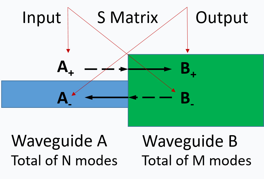
By projecting the above two boundary condition equations onto an orthogonal basis in the power inner product space, the S-matrix at the interface between waveguide A and waveguide B can be derived and thus the transmission and reflection relations between the input/output modes can be calculated:

$$\begin{bmatrix} A_{-} \\ B_{+} \end{bmatrix} = S^{interface}\begin{bmatrix} A_{+} \\ B_{-} \end{bmatrix} = \begin{bmatrix} R_{AB} & T_{BA} \\ T_{AB} & R_{BA} \end{bmatrix} \begin{bmatrix}A_{+} \\ B_{-} \end{bmatrix}$$

Here, $A_{+}=(a_{1}^+, a_{2}^+, ..., a_{M}^+)^T$ and $A_{-}=(a_{1}^-, a_{2}^-, ..., a_{M}^-)^T$ are the mode coefficients of the forward and backward propagating eigenmodes in waveguide A, respectively. Similarly, $B_{+}=(b_{1}^+, b_{2}^+, ..., b_{N}^+)^T$ and $B_{-}=(b_{1}^-, b_{2}^-, ..., b_{N}^-)^T$ are the mode coefficients of the forward and backward propagating eigenmodes in waveguide B, respectively.

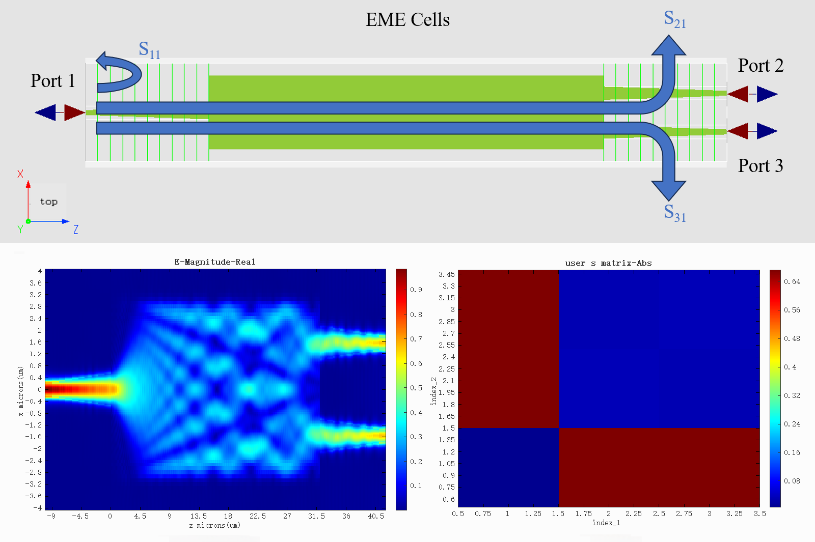
In conclusion, by solving the S-matrix for each interface and the phase transmission matrix for each cell, we can obtain the local scattering relations for each cell. Then multiple cells' S-matrices can be obtained using a cascading algorithm (e.g., Redheffer's matrix star product) to obtain the internal S-matrix of the entire device, thereby analyzing the transmission and reflection characteristics of the device. Below is the cascading formula for the S-matrices of the $i$-th and $(i+1)$-th cells:

$$S^{i,i+1} = S^{i} \star S^{i+1} \\ S^{internal}= S^{1} \star S^{2} \star ... S^{i}\star...\star S^{N}$$

Therefore, the S-matrices of the physical ports and internal ports can be calculated using the above cascading algorithm, ultimately yielding the global S-matrix of the entire system.

$$S^{user-s-matrix} = S^{left} \star S^{internal} \star S^{right}$$

References

[1] Wei-Ping Huang, "Coupled-mode theory for optical waveguides: an overview," J.Opt.Soc.Am.A 11, 963-983 (1994).
[2] Peter Bienstman, "Rigorous and efficient modeling of wavelength-scale photonic components," Ph.D. thesis, Ghent University (2001).
[3] A. W. Snyder and J. D. Love, "Optical Waveguide Theory," Chapman and Hall, London (1983).