Preface #

Directivity (formerly called directive gain) is defined as the ratio of the radiation intensity $U$ in a specified direction to the average radiation intensity $\bar U$^[1]. It is obtained through further analysis of far-field data and is one of the important parameters describing far-field radiation characteristics. This software provides the Directivity analysis group, which can further analyze and calculate the far-field results computed by the FDTD solver.

This document includes:

• Definitions and calculations of parameters such as radiated power $P_{rad}$ and directivity $D$;
• Workflow of the Directivity analysis group;
• Example: parameters such as radiated power $P_{rad}$, directivity $D$, and maximum directivity $D_{max}$ of a dipole source.

Workflow of the Directivity Analysis Group #

Full-Space Calculation Workflow #

According to the definition of directivity, the Directivity analysis group calculates directivity according to the following workflow:

graph TD;
    A[Project the frequency domain field into the far field radiation field Ecar] --> B[Convert Ecar into Esph];
    B --> C[Calculate the radiation intensity Usph];
    C --> D[Calculate the directivity Dsph];
    C --> E[Calculate the total power Prad]
    E --> F[Calculate the average radiation intensity Usph_avg];
    F --> D;

When calculating $P_{rad}$, it is assumed that all power is captured by the monitor box and that the captured power comes from the radiating antenna element itself rather than from sources outside the box. However, in practical applications, the antenna needs to be excited by an external source (referred to as the antenna feed), which must pass through the monitor box. The power carried by the antenna feed can significantly affect the calculation result. To correct for this effect, the software allows the user to specify a window around the antenna feed to subtract the power carried by the feed line. When setting the window, the size should be chosen carefully so that it captures only the input power and does not include the antenna's radiated power. In most cases, the position and size of the source window should match the source itself (for more details, refer to Coaxial-Fed Rectangular Patch Antenna). If the antenna feed itself contributes to the total radiation, the influence of the window size on directivity and radiated power should also be tested.

Grounded Calculation Workflow #

For grounded scatterers, in most cases the antenna can be considered as mounted on top of a metallic ground plane. When the ground plane is sufficiently large and the operating frequency is sufficiently low, it can be modeled as an infinite perfect electric conductor (PEC). The presence of a PEC ground plane significantly changes the radiation characteristics of the antenna system. For example, energy radiated from the antenna toward the ground plane undergoes reflection and returns, while the antenna induces currents on the ground plane, which further produce radiation.

The Directivity analysis group uses image theory to handle the infinite PEC ground plane. That is, the electromagnetic field produced by the real antenna above the ground plane can be equivalently regarded as being generated by two sources: the real antenna and its virtual image antenna. After superposition above the ground plane, the field distribution formed by these two sources is exactly the same as the original field distribution; below the ground plane, since the field inside the PEC is zero, the field distribution given by the image antenna is zero. This method is implemented by projecting a set of monitors above the ground plane into the negative half-space (-z), which is equivalent to placing a set of monitors below the ground plane and projecting them into the positive half-space (+z). Therefore, even though the induced currents on the infinite PEC ground plane contribute to radiation outside the monitor box, a finite-sized monitor box can be used to capture all radiated fields.

Therefore, for grounded scatterers, the calculation workflow of directivity is basically the same as in the ungrounded case, and the main difference lies in the treatment of the ground plane. Since the field below the infinite PEC ground plane (z<0) is zero, there is no need to place monitors in that region during simulation. To obtain the complete full-space directivity, it is necessary to use the image principle to project the near-field data captured by monitors on the non-ground plane into the z<0 region (where the range of $\theta$ is $[0, 90^\circ]$), thereby completing the far-field distribution in the lower half-space. The sum of the far-field contribution from the upper half-space and the mirrored far-field contribution from the lower half-space gives the complete radiation field directivity. The calculation workflow is as follows:

graph TD;
    A[Project the near field into far field Ecar] --Superimpose far-field projection of non-ground plane monitors and their mirrored far-field projection--> B[Calculate far-field radiation Esph];
    B --> C[Calculate the radiation intensity Usph];
    G[Calculate net transmissivity T] -.Obtain source power.-> H[Calculate radiated power Prad];
    C --> D[Calculate the directivity Dsph];
    C --integration--> F[Calculate average radiation intensity Usph0];
    F --> D;
    H -.-> D;

Other Parameter Definitions and Details #

Directivity Components #

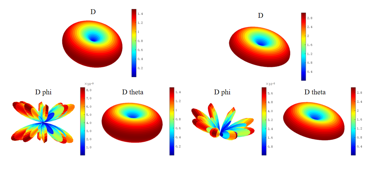
Similar to far-field data, in spherical coordinates the directivity $\boldsymbol{D}(r, \theta, \phi)$ also has no radial component $D_r$; therefore, the software only displays $D_\theta$ and $D_\phi$. For cases where $D_r$ is not zero, it is usually because the far-field condition is not satisfied. In such cases, performing a direct simulation of the project will yield more accurate results.

Symmetry and Symmetric Boundaries #

When the simulation project has good symmetry, symmetric boundaries can be used to improve simulation efficiency. However, because the near field of the complete symmetric space cannot be obtained directly, symmetric boundaries can bring some difficulties to post-processing.

For mirroring near-field data, the usual approach is to mirror the complete near-field result according to the symmetry relationship; in addition, since far-field calculation results have good symmetry, the mirror relationship can also be applied to the near-field-to-far-field projection process. These two approaches are essentially equivalent in effect and have similar computational efficiency, and both have been implemented in the software's Directivity analysis group.

Radiation Patterns and Polar Plots #

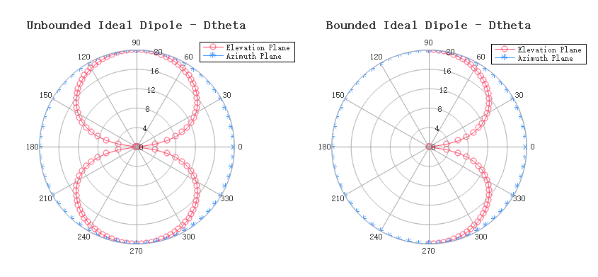
Directivity data are directly derived from the far field, so they can be intuitively presented using radiation patterns. Radiation patterns are the most common way to display far-field distributions, but understanding three-dimensional radiation patterns is often difficult. When users are only interested in a particular plane, polar plots can be used for display and analysis; if only a few specific angles are of interest, it is necessary to understand the relationship between radiation patterns and polar plots. Relevant details can be found in the examples later in this document.

Test Case: Radiation Directivity of Full-Space/Grounded Dipoles #

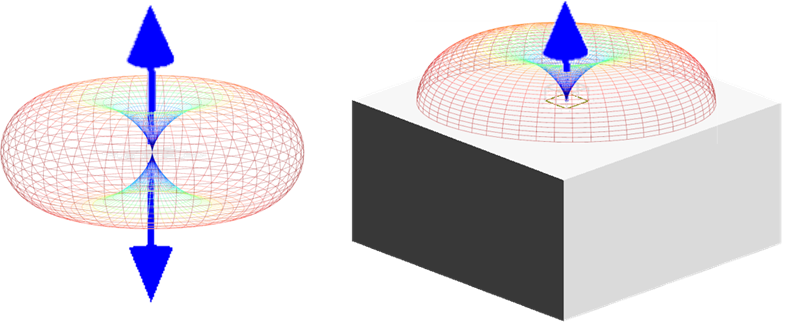
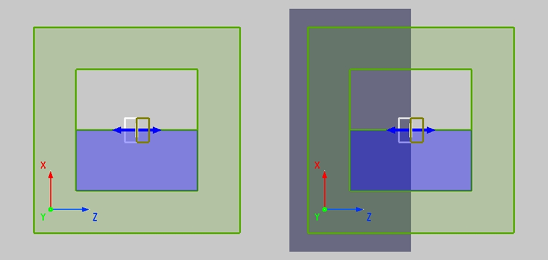
This test case calculates the radiation directivity of a dipole in full space and in the grounded case, as shown in the following figure:

The calculation results are as follows:

For a fixed plane, the following result can be obtained:

Appendix #

Relevant Parameters and Calculation Methods #

1. Radiation intensity $U$

   Radiation intensity $U$ is the power radiated by the antenna per unit solid angle in a specified direction $(\theta,\phi)$, expressed in watts per unit solid angle (W/unit solid angle). It is calculated as:

   $$U(\theta,\phi) = \frac{1}{2\eta}[|E_\theta|^2 + |E_\phi|^2]$$

2. Radiated power $P_{rad}$

   Radiated power $P_{rad}$ is the total power radiated by the antenna into space, expressed in watts (W). It is equal to the integral of radiation intensity over the entire sphere:

   $$P_{rad} = \iint_\Omega U(\theta,\phi) d\Omega$$

   where $\Omega$ denotes the full solid angle.

3. Average radiation intensity $\bar U$

   Average radiation intensity $\bar U$ is the power per unit solid angle obtained when the total radiated power is uniformly distributed over the entire sphere. It is defined as:

   $$\bar U = \frac{P_{rad}}{4\pi}$$

   It corresponds to the radiation intensity of an ideal isotropic source.

4. Directivity $D$

   Directivity $D$ is defined as the ratio of radiation intensity $U$ to average radiation intensity $\bar U$:

   $$D \equiv \frac{U}{\bar U}$$

   In this software, the directivity can be obtained directly by using the Directivity analysis group.

   If $U_{max}$ denotes the maximum radiation intensity, the maximum directivity is:

   $$D_{max} = \frac{U_{max}}{\bar U}$$

   In addition, partial directivity is defined as the ratio of the radiation intensity in a given polarization to the average radiation intensity over all directions. In spherical coordinates, since the far-field radiation contains only $E_\theta$ and $E_\phi$ ($E_r \approx 0$), the total directivity can be expressed as:

   $$D = D_\theta + D_\phi$$

References #

References

C. A. Balanis, Antenna Theory and Design, 4th Edition. John Wiley & Sons (2016). ↩︎