Settings for Plane and Gaussian Sources #

This section describes settings for plane and Gaussian sources.

Select Plane or Gaussian in solver tab and create a plane source or Gaussian source in Composite viewer. Then, set further parameters in the Edit properties interface that automatically pops up.

Settings for Plane Sources #

General Settings #

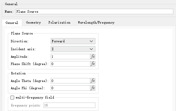
The General tab is used to set information such as the injection axis and amplitude of the source. By editing Angle theta and Angle phi , the injection angle of the source can be set. Note that Angle phi is only available in 3D simulations.

Name	Description
Direction	Incident direction of a plane source, specifically selected as Forward (forward propagation) or Backward (backward propagation).
Incident axis	Select desired incident axis for a plane source from drop-down list.
Amplitude	Source amplitude is set as 1 by default.
Phase shift	Used to set phase delay between multiple sources.
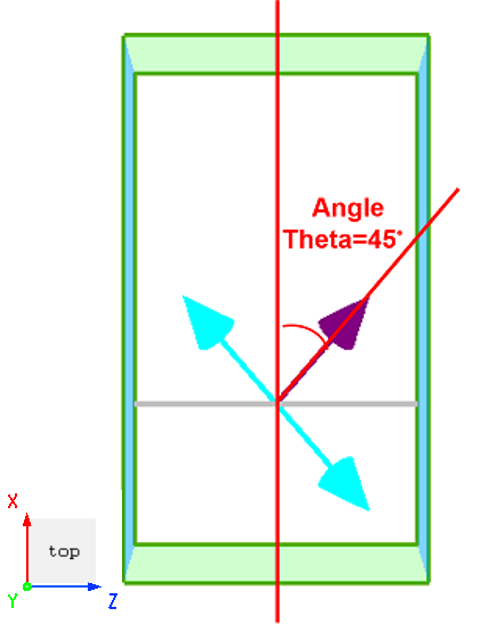
Angle theta	Polar angle. Angle between direction of source propagation and normal of incident plane.
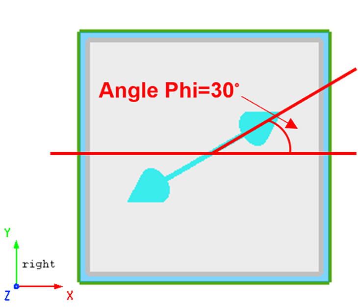
Angle phi	Azimuthal angle. Angle between projection of source in propagation direction onto interface (if light propagates along Z-axis, XY plane represents interface) and positive X-axis.

If Angle theta is set to 45 for a plane source with propagation direction in the positive Z-axis direction, ZX plane view is shown in the following figure:

If Angle phi for a plane source is set to 30, YX plane view is shown in the following figure:

Multi-frequency field is an advanced setting that can be disabled for simulation projects where source bandwidth is narrow.

Name	Description
Multi-frequency field	Multi-frequency option allows users to solve propagation characteristics of a source at multiple frequencies in optical devices. It is recommended to use this feature for broadband time-domain simulations and simulations involving injection of sources into dispersive materials, especially at a specific angle.
Frequency points	Specify number of frequencies to be used in calculation of optical field distribution, and set this value to at least 5 in order to ensure accuracy.

Geometry #

Geometry tab can be used to set geometric range of a source.

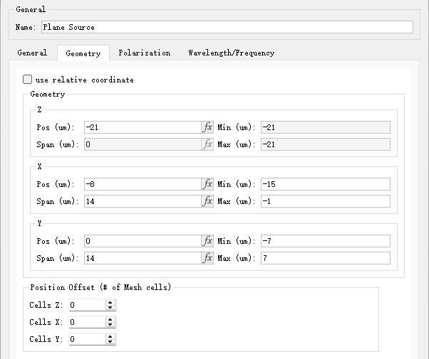
Name	Description
Use relative coordinate	Use relative coordinates.
Z/X/Y pos	Center of a source.
Z/X/Y span	Range of a source.
Cells Z/X/Y	Number of offset units in the Z/X/Y direction.

Polarization #

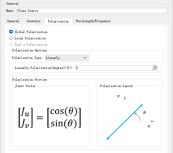
Polarization tab can be used to set polarization of a source. See Polarization below.

Wavelength/Frequency #

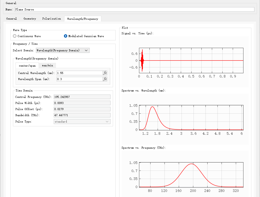
Wavelength/Frequency tab can be used to set wavelength/frequency of a source.

Name	Description
Continuous wave	Continuous wave.
Modulated gaussian wave	Modulated Gaussian wave.
Select domain	Select Wavelength or Time as the domain of input parameter.
Center/Span	Center/Span Used to set center wavelength and wavelength bandwidth.
Max/Min	Max/Min Used to set maximum and minimum values for bandwidth.
Central frequency	Define central wavelength.
Pulse width	Define pulse width which covers the wavelength or frequency range to be simulated.
Pulse offset	Defines pulse offset, i.e., time interval between start of the simulation and center of input pulse. Thus, the initial field is close to zero at the start of the simulation. To avoid interruption of the input pulse, the pulse offset should be at least twice the pulse duration to ensure that the frequency distribution is approximately symmetrical near the central frequency of the source.
Bandwidth	Define full width at half maximum (FWHM) of source in frequency domain.
Pulse type	Two types are available: Standard and Broadband. This is a read-only parameter.

Software provides wavelength/frequency domain images, which are plotted respectively for:

• Time domain signals;
• Wavelength domain spectrum;
• Frequency domain spectrum.

More Information about Plane Sources #

• If plane source is required to maintain an ideal plane wave, boundary conditions must be set as Periodic or Bloch according to specific project requirements;
• For projects involving plane sources with PML boundary conditions at the propagation direction, plane source diffracts at the edges;
• In broadband simulations, actual incident angle (non-zero angle) varies with frequency, and thus accurate results require both frequency sweeps and angle sweeps.

Settings for Gaussian Beam #

A Gaussian beam in fundamental mode is expressed as:

$$E(\rho,z) = \frac{A_0w_0}{w(z)}exp(-\frac{\rho^2}{w^2(z)})exp\{-i\{{k[\frac{\rho^2}{2R(z)}+z]-\Psi(z)}\}\}$$

where $\rho=\sqrt{x^2+y^2}$, the propagation direction is along the z-axis. $|A_0|$ is the maximum amplitude of the electric field, $w(z)$ is the spot radius of the Gaussian beam, and $w_0$ is the beam radius at the waist, which is also the minimum spot radius. $R(z)$ is the radius of curvature of the wavefront, and $\Psi(z)=tan^{-1}(\cfrac{z}{z_0})$, where $z_0$ is called the collimation distance, which is the distance at which the Gaussian beam radius expands to $\sqrt{2}w_0$.

General Settings #

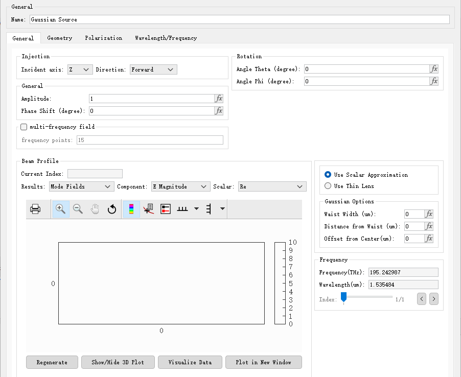
General tab can be used to set parameters of a Gaussian source, such as phase, amplitude, and beam profile.

Source Injection, Rotation, and Phase Shift #

The Injection tab is used to set the injection axis and direction of the light source, the Rotation tab is about the setting of rotation, and the General tab is about the setting of the injection amplitude and phase shift of the light source.

	Name	Description
Injection	Incident axis	Incident axis of a Gaussian source (normal to incident plane).
	Direction	Propagation direction of a Gaussian source, specifically selected as Forward (forward propagation) or Backward (backward propagation).
Rotation	Angle theta	Polar angle. Angle between direction of source propagation and normal of incident plane.
	Angle phi	Azimuthal angle. Angle between projection of source in propagation direction onto interface (if light propagates along Z-axis, XY plane represents interface) and positive X-axis.
General	Amplitude	Source amplitude is set as 1 by default.
	Phase shift	Used to set phase delay between multiple sources.

Multi-Frequency #

Multi-frequency field is an advanced setting that can be disabled for simulation projects where source bandwidth is narrow.

Name	Description
Multi-frequency field	Multi-frequency option allows users to solve propagation characteristics of a beam at multiple frequencies in optical devices. It is recommended to use this feature for broadband simulations and simulations involving injection of sources into dispersive materials, especially at a specific angle.
Frequency points	Specify number of frequencies to be used in calculation of optical field distribution, and set this value to at least 5 in order to ensure accuracy.

Visualization of Gaussian Beam #

Beam profile tab can be used to plot field distribution of a Gaussian Source.

Name	Description
Current index	The (maximum) refractive index of incident surface; a read-only parameter.
Results	Allows users to specify desired type of data to be plotted by selecting either Mode fields or Index from the drop-down list.
Components	When selecting Mode fields under Results, available components are as follows: E Magnitude, Ex, Ey, Ez, H Magnitude, Hx, Hy, and Hz. If Index is selected under Results, available components are Index_x, Index_y, and Index_z.
Scalar	Abs: modulus of selected component; Re: real part of selected component; Im: imaginary part of selected component; Phase: argument of selected component.
Regenerate	Regenerate images.
Show/Hide 3D plot	Show/hide 3D plots.
Visualize data	Open Data visualizer window.
Plot in new window	Plot image in a new window.

Settings for Gaussian Beam #

The software provides two types of Gaussian source, one for Gaussian beams using scalar approximation and the other for tightly focused Gaussian beams using thin lenses. The highly focused Gaussian beam is a fully vectorial beam. After the parameter settings are completed, users can view the current field distribution in the visualization of Gaussian beam. When the waist radius is several times larger than the wavelength used, the scalar approximation option should be selected. When the waist radius is the same as the wavelength, the thin lens option should be used.

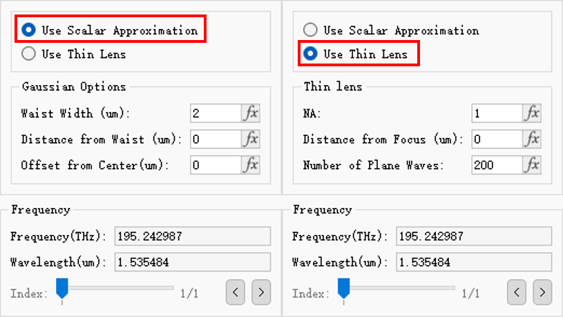
Gaussian beam with scalar approximation #

Gaussian options tab can be used to set parameters related to a Gaussian source.

Name	Description
Waist width	Waist width.
Distance from waist	Distance between incident plane and waist.
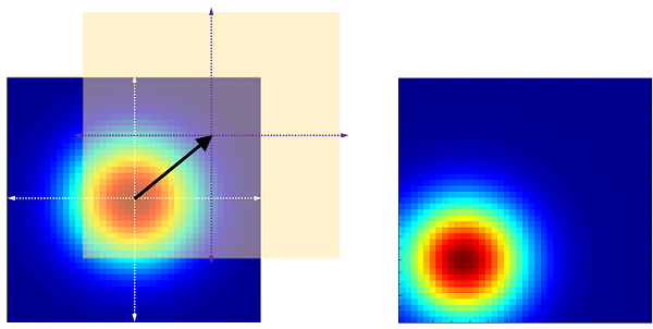
Offset from center	Transverse offset from the center of waist width.

Note:

• A Gaussian beam in fundamental mode is a symmetric distribution field centered around optical axis. Equation $\rho = \sqrt{x^2 + y^2}$ (assuming propagation direction is $z$) represents coordinates in incident plane, and parameter Offset from center refers to offset between center of incident optical field and center of Gaussian beam.
• A Gaussian beam in fundamental mode is a model that satisfies paraxial approximation conditions and is not suitable for accurately describing non-paraxial situations (a paraxial approximation must typically satisfy $\lambda << w_0$, which in simulation requires at least $\lambda \approx w_0$).

Tightly focused Gaussian beam #

The following is a tightly focused Gaussian beam by using a thin lens. The Thin lens tab allows users to set lens related parameters.

Name	Description
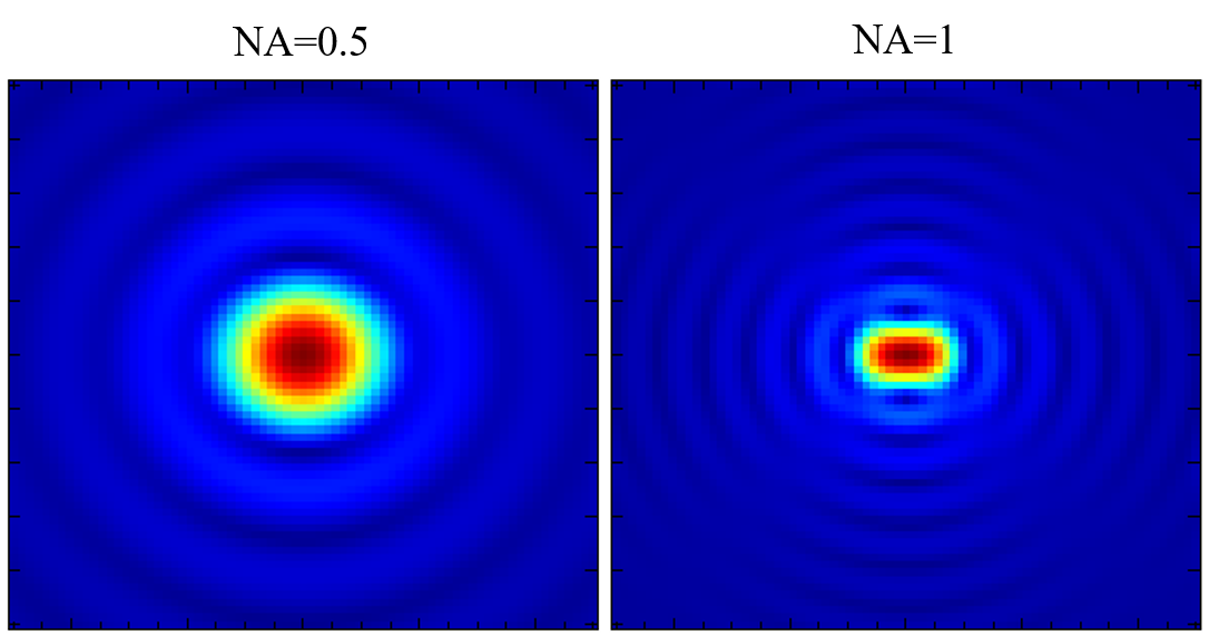
NA	The numerical aperture of a thin lens is $n*sinA$, where $n$ is the refractive index at the position of the source and A is the half angle. The following figure shows the field distribution of Gaussian source at different numerical apertures.
Distance from focus (um)	The distance between the injection plane and the focal point of the lens, where a positive number represents a diverging beam and a negative number represents a converging beam.
Number of plane waves	The number of plane waves used to construct the beam. Increasing the number of plane waves will result in a more accurate beam profile but will also increase the computation time.

Geometry #

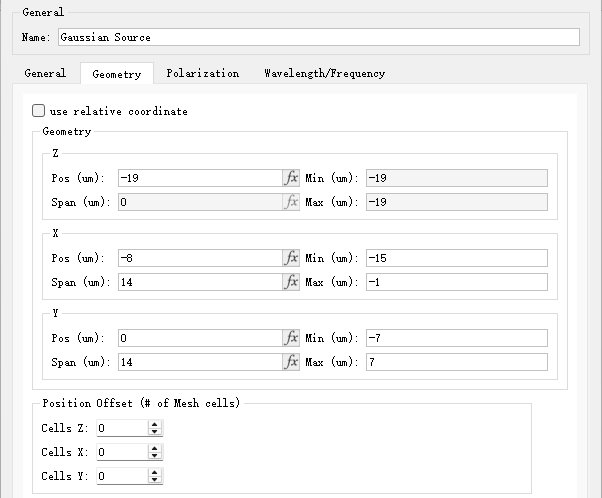
Geometry tab can be used to set geometric range of a source.

Name	Description
Use relative coordinate	Use relative coordinates.
Z/X/Y pos	Center of a source.
Z/X/Y span	Range of a source.
Cells Z/X/Y	Number of offset units in the Z/X/Y direction.

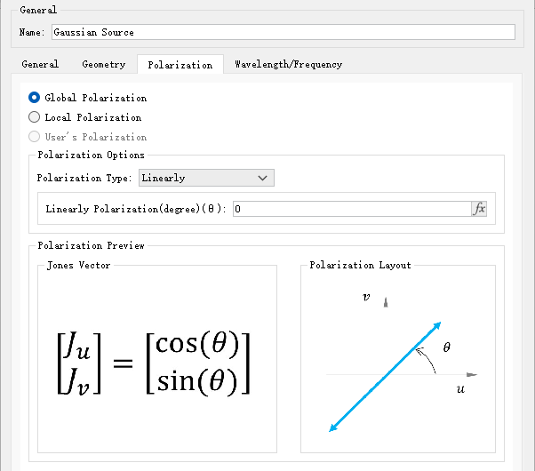
Polarization #

Polarization tab can be used to set polarization of a source. See Polarization below.

Wavelength/Frequency #

Wavelength/Frequency tab can be used to set the wavelength/frequency of a source.

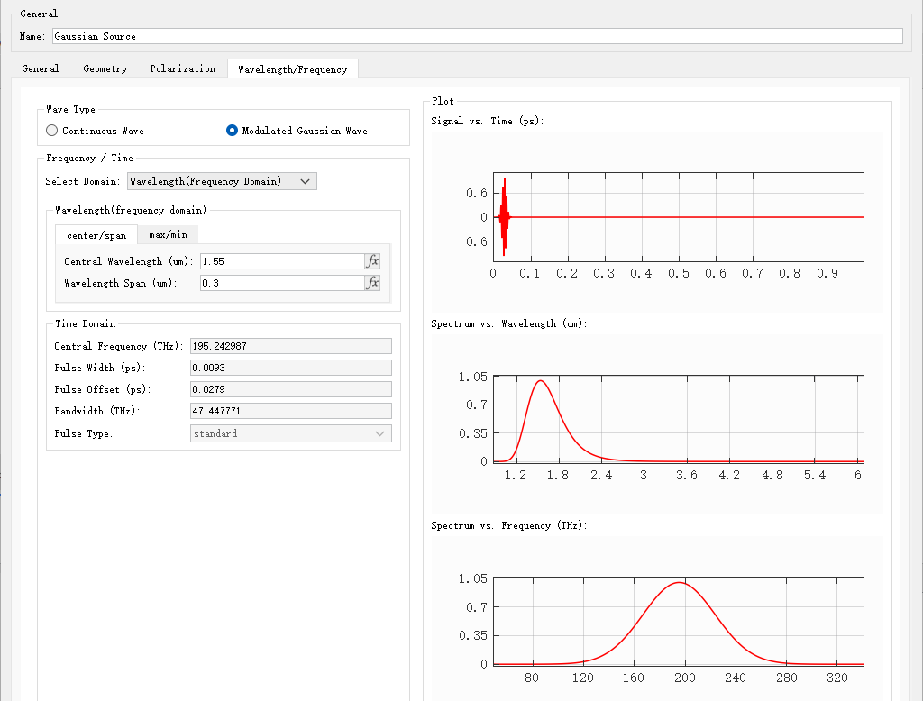
Name	Description
Continuous wave	Continuous wave.
Modulated gaussian wave	Modulated Gaussian wave.
Select domain	Select Wavelength or Time as the domain of input parameter.
Center/Span	Center/Span Used to set center wavelength and wavelength bandwidth.
Max/Min	Max/Min Used to set maximum and minimum values for bandwidth.
Central frequency	Define central wavelength.
Pulse width	Define pulse width which covers the wavelength or frequency range to be simulated.
Pulse offset	Defines pulse offset, i.e., time interval between start of the simulation and center of input pulse. Thus, the initial field is close to zero at the start of the simulation. To avoid interruption of the input pulse, the pulse offset should be at least twice the pulse duration to ensure that the frequency distribution is approximately symmetrical near the central frequency of the source.
Bandwidth	Define full width at half maximum (FWHM) of source in frequency domain.
Pulse type	Two types are available: Standard and Broadband. This is a read-only parameter.

Software provides wavelength/frequency domain images, which are plotted respectively for:

• Time domain signals;
• Wavelength domain spectrum;
• Frequency domain spectrum.

Polarization for Planar and Gaussian Sources #

Local and Global Polarization #

Polarization is a parameter typically associated with plane sources. FDTD solver allows users to define complex polarization states for a Gaussian source.

The following polarization types are available for Plane and Gaussian sources:

• Global polarization: Refers to a situation where polarization characteristics are consistent at each point on incident plane. It can be represented by a single Jone vector. Typical options provided in software include: Linear polarization, Left/Right-handed circularly polarized, Left/Right-handed elliptically polarized, etc.;
• Local polarization: Refers to a situation where polarization characteristics are different at each point on incident plane. Typical polarization characteristics provided in software include: Radial polarization, Angular polarization, Vortex polarization, and Arbitrary polarization;
• User‘s polarization: To be defined by user.

Polarization Settings #

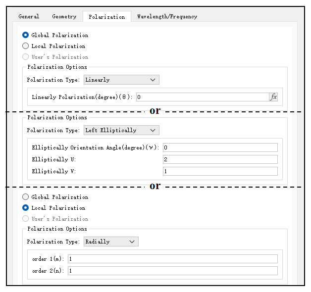
Name	Description
Linearly polarization(θ)	Define polarization angle for linear polarization.
Elliptically orientation angle	Define elliptically orientation angle for left/right-handed elliptical polarization.
Elliptically U	Define length U of first elliptical axis for left/right-handed elliptical polarization.
Elliptically V	Define length V of second elliptical axis for left/right-handed elliptical polarization.
Order 1	Define first radial order for radial/angular/vortex polarization.
Order 2	Define second radial order for radial/angular/vortex polarization.

Case: Define Circular Polarization #

Define plane wave for left-handed circular polarization:

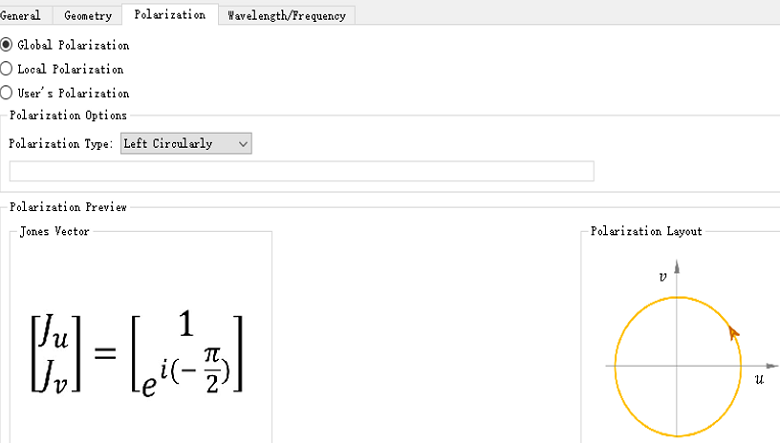
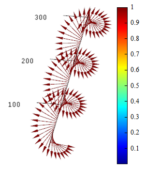
Vector is used to plot electric field vector of light in the transmission direction. As shown in figure below, electric field vector exhibits an obvious circular trajectory in transmission direction.