PML #

Perfectly Matched Layer (PML) is used to absorb electromagnetic waves incident on or reflected from the simulation boundary, reducing the influence of boundary reflections on the numerical solution. It is one of the most common absorbing boundary conditions in FDTD simulations and is especially useful for open-domain, near-field, far-field, and scattering problems.

Basic concept #

PML (Perfectly Matched Layer) is not a hard-wall boundary condition. Instead, it is an artificial absorbing layer placed outside the computational domain to reduce reflection from the simulation boundary and attenuate the electromagnetic field as it propagates into that layer. The purpose is to approximate an open, effectively infinite space so that energy leaving the domain does not return and contaminate the solution.

The underlying idea is based on stretched-coordinate or complex-parameter formulations: near the boundary, the wave is gradually damped by a controlled loss profile so that the field decays exponentially within the PML. In practice, this means the PML acts as a lossy transition region, suppressing reflections without forcing the field to vanish abruptly at the boundary.

PML effects #

Use an FDFP monitor to observe the attenuation of the field as it passes through the PML. The recorded field amplitude typically decreases rapidly with distance inside the PML, indicating that the wave energy is being absorbed by the layer rather than reflected back into the domain.

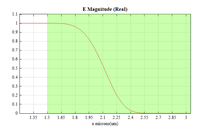
As shown in the figure, once light enters the PML, the field decays layer by layer and eventually becomes negligible. This is the main objective of an absorbing boundary: to maintain an accurate open-domain response while avoiding artificial reflections from the outer boundary.

PML and structure #

The software uses a stretched-coordinate PML. For structures that pass through the PML boundary, refer to the related boundary discussion on the Structure page. In the FDTD boundary condition settings, there is an option labeled Extend Structure through PML, as shown below. This option is enabled by default.

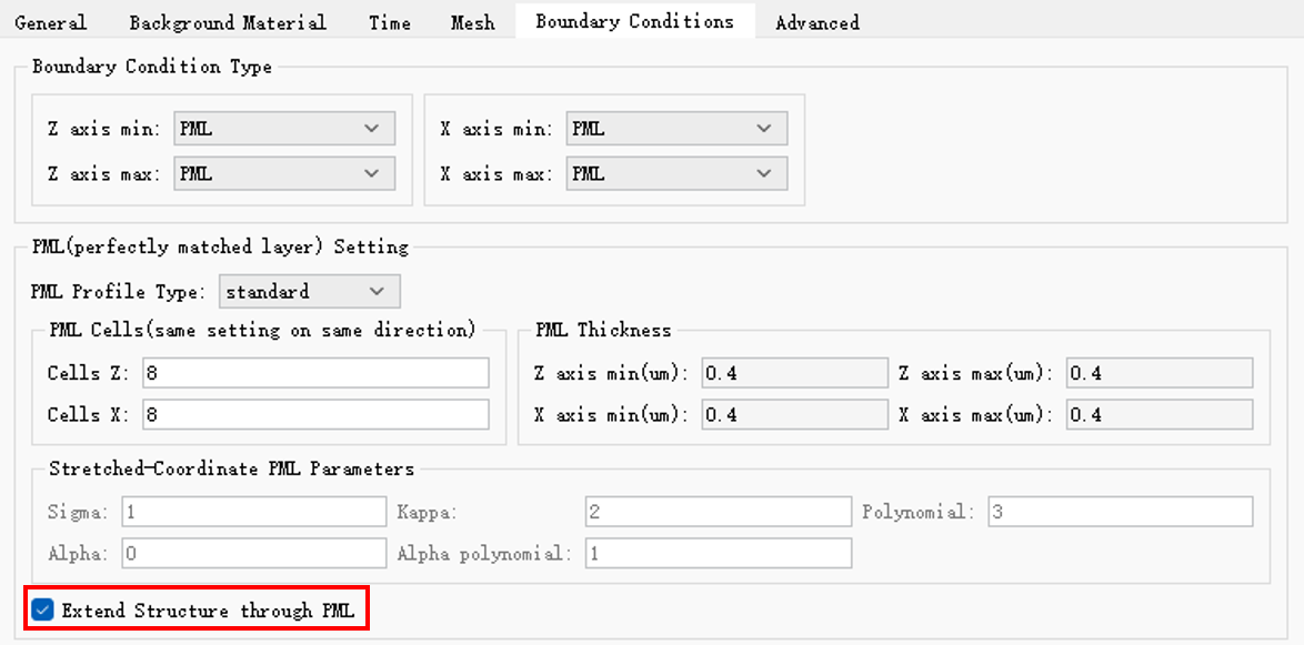
When this option is enabled, the software automatically extends the structure that touches the inner PML boundary in the direction normal to the boundary. For multilayer slabs or other structures directly adjacent to the boundary, this usually reduces reflection and improves absorption performance.

However, for periodic structures such as photonic crystals, this option should generally be disabled. Extending a periodic crystal that touches the inner boundary would alter the periodicity near the edge and produce an artificial, nonphysical boundary condition.

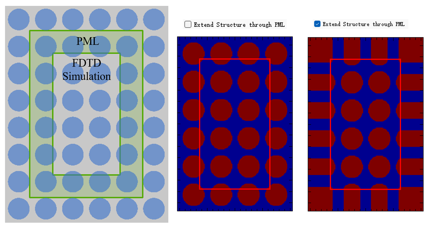
When PML is used as an absorbing boundary, it is important to keep a sufficient buffer region between the main structure of interest and the simulation boundary so that residual reflections do not contaminate the target field distribution. If the structure, source, or observation region is too close to the PML, or even extends into the PML layer, then the model may need a larger computational domain, a thicker PML, or a different boundary condition choice. For periodic systems that require translational symmetry, special care should be taken not to artificially extend the structure near the boundary, since this can break the physical assumptions of the model.

PML configuration types #

The performance of PML depends strongly on the selected configuration type. The software provides three predefined PML profiles to balance absorption efficiency, numerical stability, and computational cost. Users can choose the appropriate profile from the PML profile type drop-down menu.

Name	Description
Standard	This profile provides good overall absorption with relatively few layers and is the default choice for most routine simulations. It is suitable when the structure does not pass through the PML region.
Stabilized	This profile is designed for cases where material interfaces cross the PML layer or the source is incident on the PML at a large angle. It improves numerical stability by adjusting the PML parameters and increasing the number of PML layers, which reduces the risk of field divergence inside the absorbing layer.
Custom	This profile allows users to directly specify PML parameters. The default values are based on the Standard configuration. It is recommended only for users who understand the physical impact of these parameters and need finer control.

In most cases, Standard is the preferred starting point. If the boundary region involves strong material transitions or high-angle incidence, Stabilized is usually more robust. Custom should be used only after the user understands how each parameter changes the profile and absorption depth.

PML parameter settings #

The absorption performance of PML is controlled by a set of parameters that determine the loss profile and the effective impedance match between the computational domain and the absorbing layer.

For the Custom profile, the following parameters can be specified:

Name	Description
Cells Z/X/Y	The number of PML cells, which determines the layer thickness and absorption range.
Sigma	The conductivity of the PML layer, which controls the attenuation strength of the field inside the layer.
Alpha	The loss coefficient of the PML layer, which helps reduce reflection from low-frequency or low-angle components.
Kappa	A dimensionless parameter used to adjust the effective material properties and impedance matching in the PML.
Polynomial	A polynomial function used to describe the spatial variation of Kappa and Sigma.
Alpha polynomial	A polynomial function used to describe the spatial variation of Alpha.

For the Standard or Stabilized profile, the main user-adjustable parameter is:

Name	Description
Cells Z/X/Y	The number of PML cells, which affects the thickness and stability of the absorbing layer.

In general, increasing the PML thickness and selecting a suitable profile improves absorption, but it also increases the computational cost. A balanced setting is recommended to maintain both accuracy and efficiency.

Applicable scenarios #

PML is suitable for the following typical cases:

• open-space propagation problems;
• wave radiation, scattering, and transmission into or out of a bounded domain;
• near-field and far-field analyses;
• multilayer, periodic, and complex structural models with open boundary conditions.

Usage requirements #

When PML is used as an absorbing boundary, the most important requirement is to leave sufficient free space and absorption-layer thickness between the region of interest and the simulation boundary so that residual reflections near the boundary do not contaminate the target field distribution. If the structure, source, or observation region is too close to—or intersects—the PML layer, increase the computational domain, add more PML cells, or select a more stable PML profile to prevent boundary-induced errors.

For near-field, far-field, scattering, and radiation analyses, ensure there is adequate propagation distance between the structure and the boundary so that the field evolution can be recorded before the wave reaches the absorbing layer.

The simulator allows sources and monitors to extend beyond the simulation region. Note:

• By default, the part of a source that lies outside the simulation region is inactive;
• By default, monitors do not record data outside the simulation region;
• Monitors may provide an option to record PML-internal fields: Record data in PML.

Notes #

• PML is the preferred absorbing boundary for many open-region problems, but it is not universal: if the structure crosses the PML or the source is incident at a large angle, numerical instability can occur—consider using the Stabilized profile or increasing PML thickness.
• For structures that touch the PML, use the "Extend Structure through PML" option selectively: it helps for multilayer planar structures but should be disabled for periodic systems (e.g., photonic crystals) to preserve periodicity.
• Use the Custom profile only after understanding the effect of PML parameters; Standard is recommended for typical cases.
• Record and inspect field attenuation inside the PML (e.g., via monitors or line plots) to validate absorption and detect artificial reflections.