

Polarization Rotator
Preface
In integrated optical waveguides, asymmetric cross‑sectional geometries often lead to different propagation characteristics for the transverse electric (TE) and transverse magnetic (TM) modes. As a result, some on‑chip devices can only operate in a single polarization state. A polarization rotator (PR) utilizes a specially designed waveguide structure to accumulate the phase difference between the TE and TM modes, thereby enabling conversion between the two polarization states. This example introduces the simulation method for a polarization rotator and demonstrates two approaches for calculating the rotation length using the FDE and EME solvers.
Simulation settings
Structure Description
When two different modes propagate in a waveguide, they accumulate different phases over the same distance due to the difference in their effective refractive indices (). Let the effective indices of the two modes be and ; after a propagation length , the phase difference is given by:
When the phase difference reaches , complete conversion between the two modes is achieved, and the corresponding propagation length is:
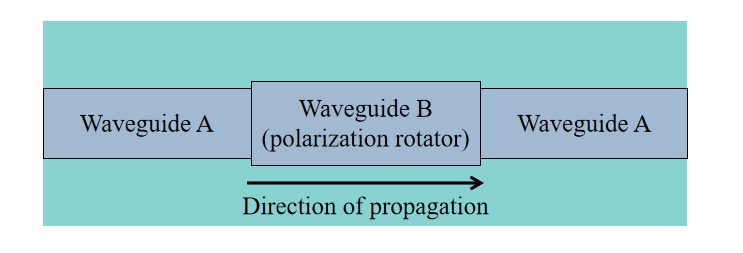
Taking waveguide A as an example, it supports both TE and TM modes with an effective index of approximately . To convert the TE mode to the TM mode, a specially designed section of waveguide B (the polarization rotator) is inserted between two segments of waveguide A, as shown in the figure above.
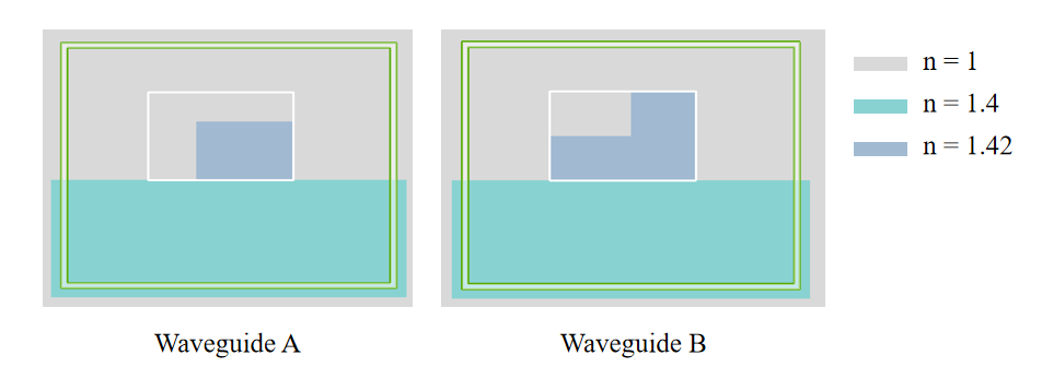
In the FDE simulation, the structures of waveguide A and waveguide B are as shown below. The simulation wavelength is . Boundary conditions are set to PEC, the mesh refinement is set to Conformal variant VP‑EP 1 with 18 refinement cells, and an additional mesh override is added with a mesh size of in both the x and y directions.
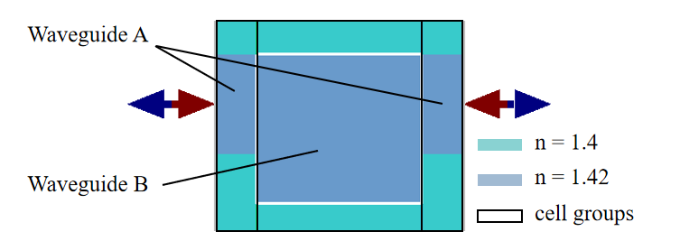
In the EME simulation, three cell groups are defined for the solver, covering waveguide A, waveguide B, and waveguide A, respectively, as shown in the figure. Since the cross‑section is uniform along the propagation direction within each group, only one cell is needed per group. The Energy Conservation option is set to Make Passive; the boundary conditions, mesh refinement, and number of refinement cells are kept the same as in the FDE simulation, and an additional mesh override is added on waveguide B with a mesh size of in the x and y directions.
Simulation Results
FDE Results
Open the waveguideA.mpps project and run the polarization_rotator.msf script (make sure user_function.msf is in the same folder). This script calculates the conversion efficiency of the polarization rotator. It first computes the eigenmodes of waveguide A and waveguide B, and then calculates the fraction of the TE mode of waveguide A that couples into each mode of waveguide B. The results are:
TE mode waveguide A has been decomposed into 2 modes of waveguide B
This accounts for 84.5272% of the incident power
Next, the script computes the propagation length required to achieve a polarization rotation (i.e., a phase difference of ) based on the effective index difference between the first two modes of waveguide B, and propagates the mode over that distance to obtain the output field distribution.
propagation of length 6.29521mm in waveguide B
Finally, the script couples the output field back into the modes of waveguide A and calculates the transmitted power in each mode. The conversion efficiency from the TE mode to the TM mode is:
After propagation of length 6.29521mm in waveguide B, we couple back to waveguide of type A and find
    17.6598% power coupling to TE mode
    67.3019% power coupling to TM mode
Total transmission from TE mode to TM mode of waveguide A is: 56.8884%
Total transmission from TE mode to TE mode of waveguide A is: 14.9273%
It should be noted that this example is intended to demonstrate the basic simulation procedure for a polarization rotator and does not optimize the structure of waveguide B. Higher polarization rotation efficiency can be achieved by optimizing the geometric dimensions of waveguide B.
EME Results
The FDE method described above can compute the optimal rotation length and efficiency, but it does not provide a continuous view of the efficiency as a function of propagation length. To observe this trend, the EME solver can be used for a sweep analysis.
Open the polarization_rotator_EME.mpps project and run the polarization_rotator_EME.msf script. The script performs a propagation sweep that scans the length of the second cell group (waveguide B) from to , and plots the results as shown below. The red curve indicates the polarization conversion efficiency from the TE mode to the TM mode.
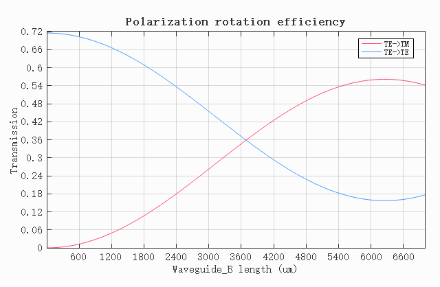
The simulation results show that the conversion efficiency from TE to TM reaches a peak of approximately at a waveguide B length of about . The table below compares the results obtained from the two solvers; they agree well, with the deviation mainly arising from the custom propagation algorithm used in FDE.
| Solver | Peak efficiency | |
|---|---|---|
| FDE | 6.295 mm | 56.89% |
| EME | 6.230 mm | 56.12% |
In the above simulation, only the first two modes of waveguide B were included. However, the TE mode of waveguide A can also expand into higher‑order modes of waveguide B. If more modes are included in the simulation, interference between the fundamental and higher‑order modes will give rise to beats. Beats refer to the periodic oscillation of transmitted power along the propagation direction, caused by interference among multiple modes with different propagation constants. The oscillation period depends on the effective index differences among the modes.
The script polarization_rotator_EME_beats.msf increases the number of modes in waveguide B and shortens the sweep length range to resolve the beat details. Running this script plots the transmission of the TE mode for different numbers of modes, clearly revealing the beats phenomenon, as shown in the figure below.
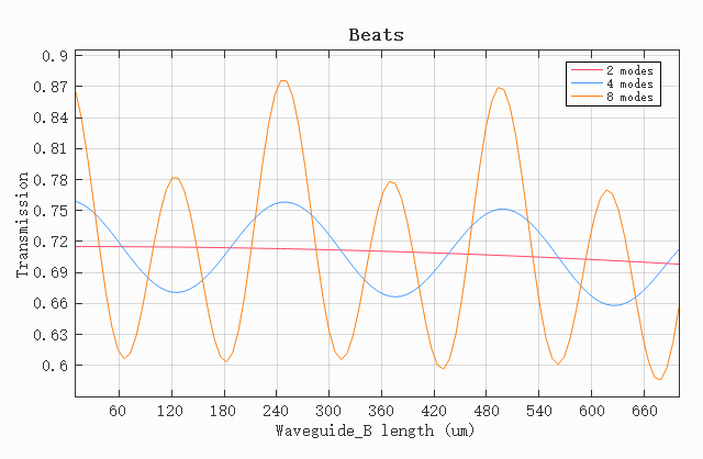
In practical designs, the presence of higher‑order modes can lead to beats, introducing additional loss and crosstalk. Therefore, the choice of the number of modes should strike a balance between computational accuracy and physical fidelity. If one only needs the envelope trend of the conversion efficiency, the first 2 modes are sufficient; for accurate analysis of device loss or bandwidth, however, more modes should be included.
