Settings for Import Sources #

This section describes settings for import sources.

Import sources offer users more flexible options, and here are some settings related to Import sources.

Select Import in the solver tab and create an Import source in Composite viewer, then set further parameters in the Edit properties interface that automatically pops up.

Settings for Import Sources #

General Settings #

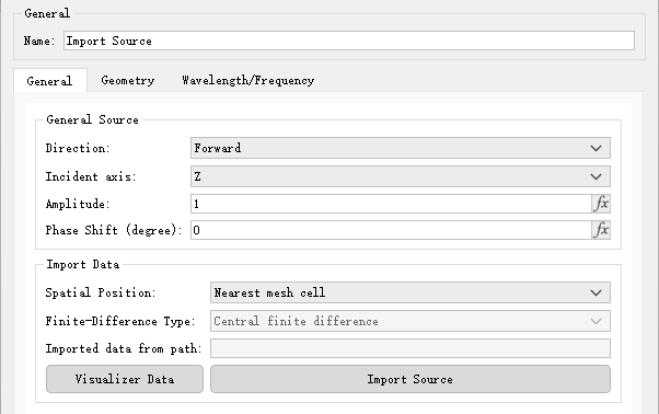
General source tab can be used to set incident axis, amplitude, and other parameters related to a source.

Name	Description
Incident axis	Select desired incident axis for an import source from the drop-down list.
Direction	Incident direction of an import source, specifically selected as Forward (forward propagation) or Backward (backward propagation).
Amplitude	Source amplitude is set as 1 by default.
Phase shift	Used to set phase delay between multiple sources.

Import data tab can be used to set parameters related to importing data.

Name	Description
Spatial position	Spatial position for importing data can be selected as either center of the mesh boundary (Yee-cell) or intersection point of the mesh (Nearest mesh cell).
Finite-difference type	Optional types include Central finite difference and Yee-cell-based finite difference.
Imported data from path	This is a read-only parameter.
Visualize data	Open the Visualizer window.
Import source	Enter interface for selecting files to be imported.

Geometry #

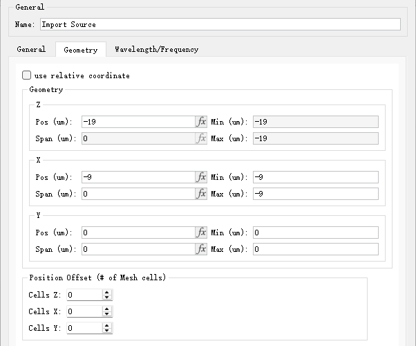
Gemetry tab can be used to set geometric dimensions of a source.

Name	Description
Use relative coordinate	Use relative coordinates.
Z/X/Y pos	Center of a source.
Z/X/Y span	Range of a source.
Cells Z/X/Y	Number of offset units in the Z/X/Y direction.

Wavelength/Frequency #

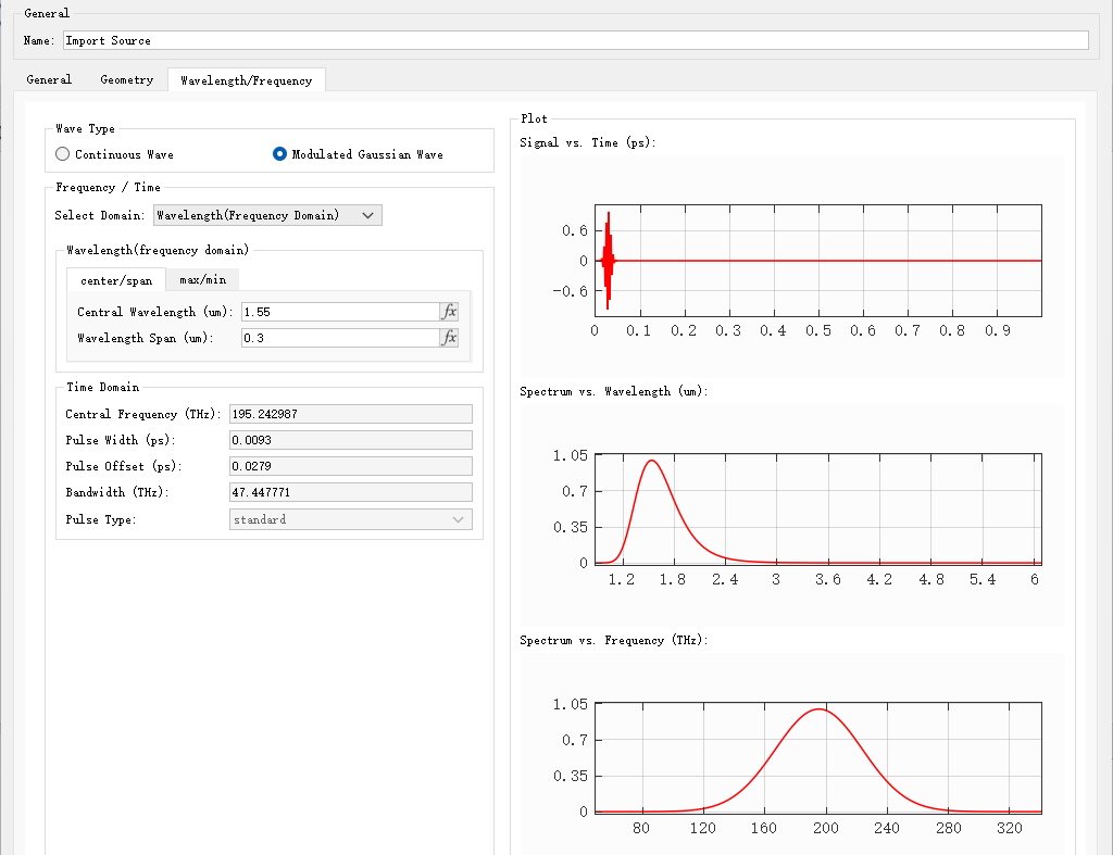
Wavelength/Frequency tab can be used to set wavelength/frequency of a source.

Name	Description
Continuous wave	Continuous wave.
Modulated gaussian wave	Modulated Gaussian wave.
Select domain	Select Wavelength or Time as the domain of input parameter.
Center/Span	Center/Span Used to set center wavelength and wavelength bandwidth.
Max/Min	Max/Min Used to set maximum and minimum values for bandwidth.
Central frequency	Define central wavelength.
Pulse width	Define pulse width which covers the wavelength or frequency range to be simulated.
Pulse offset	Defines pulse offset, i.e., time interval between start of the simulation and center of input pulse. Thus, the initial field is close to zero at the start of the simulation. To avoid interruption of the input pulse, the pulse offset should be at least twice the pulse duration to ensure that the frequency distribution is approximately symmetrical near the central frequency of the source.
Bandwidth	Define full width at half maximum (FWHM) of source in frequency domain.
Pulse type	Two types are available: Standard and Broadband. This is a read-only parameter.

Software provides wavelength/frequency domain images, which are plotted respectively for:

• Time domain signals;
• Wavelength domain spectrum;
• Frequency domain spectrum.

Case #

Construction of field data is one of the main concerns when importing sources. Software requires field data to be transferred to import sources in the fixed form.

We will demonstrate how to use import source. In this case, we first construct a Gaussian source dataset with z-axis incidence. The script is as follows:

# Define parameters;incident axis is Z
points = 201;
x = linspace(-5e-6, 5e-6, points);
y = linspace(-4e-6, 4e-6, points);
z = -4e-6;
lambda = 0.5e-6;
f = c/lambda;
index = 1;

# Calculate field components using Gaussian formula
[x0,y0] = meshgrid(x,y);
w0 = 1e-6;
f_a = exp(-((x0/w0).^2 + (y0/w0).^2));
f_a = f_a.';
Ex = f_a;
Ey = zeros(points, points);
Ez = zeros(points, points);
Hx = zeros(points, points);
Hy = f_a*sqrt(eps0/mu0);
Hz = zeros(points, points);

# Create EH dataset
Gaussian_fields = matrixdataset('fields');
Gaussian_fields.addparameter('x', x);
Gaussian_fields.addparameter('y', y);
Gaussian_fields.addparameter('z', z);
Gaussian_fields.addparameter('lambda', lambda, 'f', f);
Gaussian_fields.addattribute('E', Ex, Ey, Ez);
Gaussian_fields.addattribute('H', Hx, Hy, Hz);
Gaussian_fields.setparameterunit('x','length');
Gaussian_fields.setparameterunit('y','length');
Gaussian_fields.setparameterunit('z','length');
Gaussian_fields.setparameterunit('lambda','length');
Gaussian_fields.setparameterunit('f', 'frequency');

# Save the dataset as a .mat file
savematlabmatfile('Gaussian_fields.mat', Gaussian_fields);

Import data Gaussian_fields.mat to an Import source, run FDTD simulation, and view transmission field on the monitor, the results are as follows:

Import-E magnitude	Transmission field-E magnitude

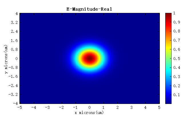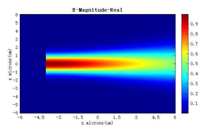Users can import any field data according to the above-mentioned data format, thereby forming a customized imported light source.