Eigenmode Expansion (EME) Solver #

The Eigenmode Expansion (EME) solver obtains the complete optical characteristics of a device by dividing a long waveguide structure into multiple computational cells along the direction of propagation. Within each cell, it solves for the eigenmodes of its cross-section, then calculates the coupling of these modes between adjacent cells.
The EME solver is particularly well-suited for analyzing and designing photonic devices whose length is much greater than the wavelength and that have slowly varying or periodic refractive index distributions. Examples include Multimode Interference (MMI) couplers, Fiber Bragg gratings, and adiabatic tapers. Compared to direct three-dimensional Finite-Difference Time-Domain (3D FDTD) simulations, the EME solver achieves extremely fast calculation speeds while maintaining accuracy. It allows for rapid scanning and optimization of key parameters such as device length and wavelength after computing the modes once, significantly enhancing the design efficiency of photonic integrated devices.

EME Solver Settings #

To add an EME solver, select the EME button in the Home tab, then click anywhere in the Composite Viewer window to create it. Modify the solver's settings in the automatically opened properties editor window to complete the setup.

The EME solver properties page is shown below and will be explained in detail in the following sections.

General Settings #

The General tab is used to configure the solver's simulation space, which includes the simulation dimension and geometry.

Simulation Dimension #

The Dimension tab is used to set the simulation dimension for the EME solver. Currently, three normal directions are supported: 2D Z normal, 2D X normal, and 2D Y normal.

Geometry #

The Geometry tab is used to set the geometric size of the EME solver region.

Name	Description
X/Y/Z pos	Sets the geometric center of the solver's simulation region.
X/Y/Z span	Sets the extent of the solver's simulation region along the three-dimensional coordinate directions.

EME Settings #

This tab contains the core settings specific to the EME algorithm, used for defining the computational cells.

Central Wavelength #

Name	Description
central wavelength	Sets the central wavelength used for calculating the eigenmodes in all cells.

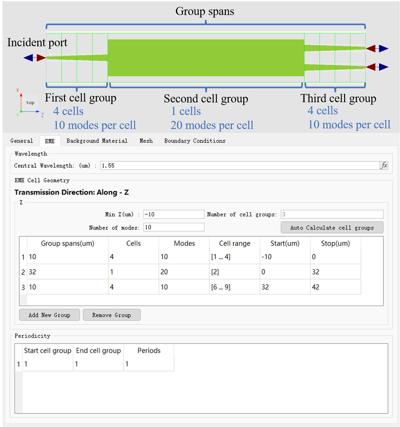
EME Cell Geometry #

This section allows you to define one or more cell groups, each of which can have independent geometry and mode settings. Key parameters in the table include:

Name	Description
Group span (µm)	The overall width of this cell group (along the propagation direction).
Cells	The number of cells this group is subdivided into. A higher number of cells typically means higher accuracy but also greater computational cost.
Modes	The number of eigenmodes calculated and used for this cell group. Must include all propagating modes to ensure accuracy.
Cell range	The range of cell indices included in this group.
Start/Stop (µm)	The start and stop coordinates of this cell group.
Display cells	When checked, displays the boundary outline of each calculation cell in the Composite Viewer; uncheck to hide. Checked by default.

Additionally, key configuration items are:

Name	Description
Energy conservation	Sets the energy conservation type for the interface S‑matrix. Supports three options: none (no conservation), passive (default; forces norm to 1 if it exceeds 1), and conserve energy (forces norm to 1, typically required for periodic structures such as Bragg gratings).
Number of modes	Sets the number of modes to solve.
Min z	Starting coordinate of the entire EME simulation region.
Number of cell groups	Defines the total number of cell groups.

Periodicity #

If your defined structure is periodic, you can view and modify the number of repetitions of the periodic unit in this section.

Name	Description
Start cell group	The starting cell group index for a periodic unit.
End cell group	The ending cell group index for a periodic unit.
Periods	The number of repetitions of the above periodic unit.

Background Material #

The Background Material tab provides a Background Material dropdown menu for selecting the background material.

Name	Description
Background material	Background materials can be selected from the built-in Optical Materials Library , or you can create custom materials and add them to the library via the Add/Edit button.

Mesh #

The Mesh tab provides the mesh settings for the solver. The EME solver offers both uniform mesh and auto non-uniform mesh settings. For specific parameters, please refer to Mesh Settings.

Boundary Conditions #

The Boundary conditions tab provides the boundary condition settings for the solver. For detailed settings of each parameter, refer to Boundary Conditions.

Advanced #

The Advanced tab contains three sections: Mesh generation , EME setting, andMode solver settings:

1. Mesh generation:

Provides forced mesh symmetry settings, allowing grid symmetry to be enforced independently in the x / y / z directions.

2. EME setting:

Provides tolerance controls to adjust the accuracy and stability of interface S‑matrix calculations, energy conservation corrections, and internal matrix solutions. The following three key tolerance control parameters are provided:

• a. Tolerance 1: Mode Coupling Truncation Tolerance

  • Functional Definition:
    This parameter is used to handle abnormal mode coupling that occurs when solving for the interface S-matrix. When there is a severe mode mismatch between the two sides of an interface (i.e., modes on one side cannot be effectively expanded on the other), the computation may yield non-physical S-parameters far greater than 1, thereby violating the passivity and energy conservation of the device. Introducing this tolerance truncates and eliminates such abnormal coupling.

  • Parameter Settings:

    • Close to 0: The mode field distribution at the interface is smoother, but it may cause severe violations of energy conservation, which are difficult to correct without perturbing the overall S-matrix.
    • Close to 1: Yields the best energy conservation correction, but the interface field distribution may exhibit discontinuities.
    • Recommended Solution: For periodic structures where precise energy conservation is critical, it is generally recommended to set this value between $0.5 \sim 1$.

  • Note:
    Regardless of whether the Energy Conservation option is enabled, this parameter affects the calculation of all interface S-matrices.

• b. Tolerance 2: Energy Correction Tolerance

  • Functional Definition:
    This parameter establishes the minimum power threshold at which the system is allowed to apply corrections during the energy conservation process. When the Conserve Energy option is enabled, the system automatically compensates for modes that exhibit numerical loss.

  • Parameter Settings:
    For periodic structures where exact energy conservation is important, it is recommended to set this to a small value, such as $10^{-3}$ or lower, to prevent erroneous corrections.

  • Note:
    This parameter is only active when Energy Conservation is set to Conserve Energy.

• c. Tolerance 3: Numerical Stability Tolerance

  • Functional Definition:
    This parameter is designed to suppress ill-conditioned behavior during matrix operations when computing the interface S-matrix, ensuring the stability and reliability of the numerical results. It works by filtering out non-physical singular components caused by minor numerical perturbations, limiting excessive amplification effects during matrix inversion.

  • Parameter Settings:
    It should typically be kept at a relatively small value (e.g., $10^{-2}$ or lower) to ensure it does not interfere with normal physical coupling. If set too high, it may artificially flatten out weak but genuine mode correlations.

  • Note:
    This parameter is active when the Energy Conservation option is set to Conserve Energy or Make Passive.

3. Mode solver settings:
Mode solver settings are used to set the material data sampling method, including the following two options. This part of the settings is basically the same as the FDE settings. For details, please refer to FDE Advanced.

Name	Description
Linear interpolation	When applying the Linear interpolation to acquire material data, the resulting material data may have discontinuities in frequency.
Fit model	Use a polynomial material model to fit Sampled material data.