Preface #

The directional coupler is one of the most fundamental and widely used passive components in silicon photonic integrated circuits. It exploits the evanescent-wave coupling effect between two parallel waveguides to extract or distribute optical power in a designed proportion and direction, without interrupting the main signal transmission. This device is not only a core unit for on-chip optical power splitting, signal monitoring, and feedback control, but also a basic building block for larger-scale functional devices such as Mach–Zehnder interferometers and microring resonators. In high-end silicon photonic chip design, the accuracy of the coupling ratio of a directional coupler directly determines the insertion loss, crosstalk, and signal integrity of the entire link. Therefore, accurately predicting its coupling ratio through FDTD simulation is a critical prerequisite for successful design. Different FDTD simulation software may differ in implementation details such as mesh generation, material boundary treatment, and conformal mesh algorithms. Based on the directional coupler described in Section 3.1 of Liu [1], this work demonstrates through reasonable variable control that the three software tools agree closely on key performance indicators.

Simulation settings #

Device introduction #

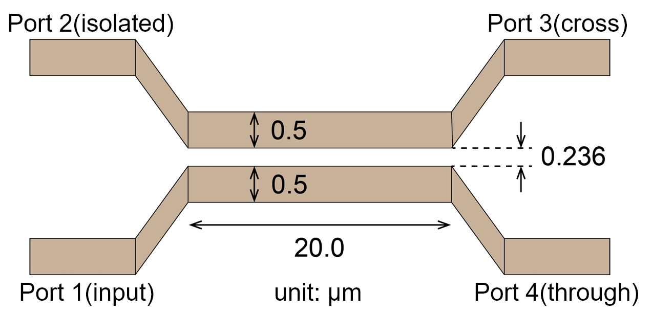
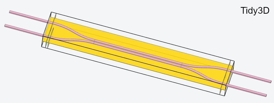
The directional coupler structure used in this work refers to the design in Section 3.1 of Liu . Specifically, it consists of two 500 $nm$ wide and 220 $nm$ high silicon waveguides placed in close proximity within a 20 $μm$ long coupling region, with a gap of 236 $nm$. The top and bottom of the device are cladded with silicon dioxide. Port 1 serves as the input port, Port 3 as the coupling port, and Port 4 as the through port. To ensure that the input and output waveguides extend through the boundaries in the propagation direction and yield reliable results, each port is extended by a 10 $μm$ long straight waveguide.

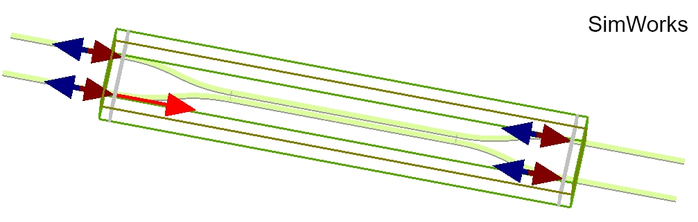
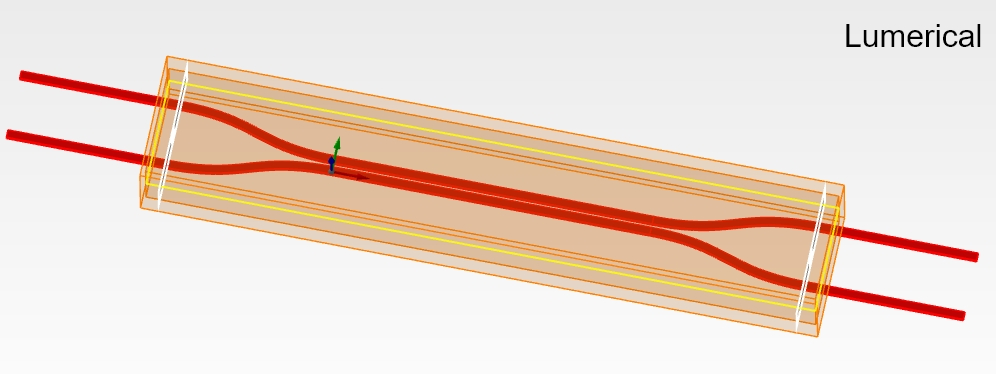
Following the setup of the paper, the incident light is the fundamental TE mode at a center wavelength of 1550 $nm$, with a bandwidth of 20 $nm$ or 50 $nm$. The mesh type is semi‑automatic non‑uniform, with the mesh defined in terms of the number of cells per wavelength; its value is 15 cells per wavelength. The simulation domain size is 42×7×4 $μm³$. The positions of the source and monitors, as well as the PML boundary conditions, are exactly the same across the three software tools. The auto‑shutoff ratio is set to 1e-5 for early shutoff. For materials, both SimWorks and Lumerical employ Si‑Palik (sampled data), while Tidy3D uses a pole‑residue model. The 3D views of the three software tools are shown below.

Simulation results #

Results under the Paper’s Settings #

First, the directional coupler is simulated using exactly the settings described in the paper, i.e., a dispersive material model, semi‑automatic non‑uniform mesh (15 cells per wavelength), and the respective default conformal mesh treatment. The figure below shows the simulation results of the three software tools under these conditions. The transmission obtained by the three softwares increases monotonically with wavelength. The results of Tidy3D deviate by only about 0.1% under the two bandwidths; in contrast, SimWorks and Lumerical show significant deviations under different bandwidths. This is because, although all three software tools perform the simulation at a resolution of 15 cells per wavelength, the wavelength used for mesh generation differs: Tidy3D uses the center wavelength, whereas SimWorks and Lumerical use the shortest wavelength within the bandwidth. A change in bandwidth therefore alters the automatically generated mesh, which in turn causes a slight change in the simulation results.

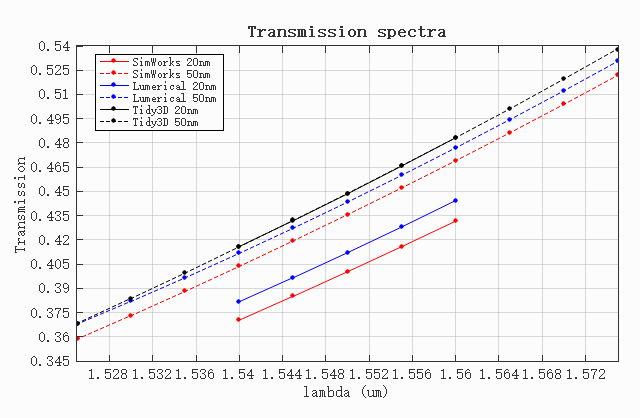
Compared with Tidy3D, both SimWorks and Lumerical yield a lower transmission for the 20 $nm$ bandwidth than for the 50 $nm$ bandwidth. Specifically, the transmission obtained by Lumerical at a bandwidth of 20 $nm$ deviates by 3% from its 50 $nm$ result; its spectrum at 50 $nm$ bandwidth is closer to Tidy3D and about 0.7% lower than the latter. The results of SimWorks under different bandwidths deviate by 3.7%, and its transmission is overall lower than the other two software tools. This is because the default mesh refinement subcells in SimWorks is 5, which leads to a lower computational accuracy of the equivalent permittivity at material boundaries compared to the built‑in defaults of the other two software tools, and thus the coupling efficiency is underestimated. It will be demonstrated below that by adjusting the number of mesh refinement subcells, the results of SimWorks can be made to match those of the other two software tools.

Results with a Staircase Approximation at Material Boundaries #

In order to better compare the performance of the three software tools, a controlled‑parameter approach is adopted. First, to eliminate the slight differences arising from the fitting of material dispersion models, the materials in all three software tools are uniformly set to dielectric materials, with the refractive index of silicon set to 3.47647 and that of silicon dioxide set to 1.44568. The incident source is uniformly the fundamental TE mode at a center wavelength of 1550 $nm$, with a bandwidth of 20 $nm$ or 50 $nm$, and the multi‑frequency field injection function is not enabled. Second, to eliminate the interference caused by inconsistent mesh sizes, a uniform mesh is adopted in all three software tools, and the mesh step size is fixed at 0.02972 $μm$, which corresponds to a resolution of 15 cells per wavelength in the silicon medium. Except for the treatment of material boundaries, all other simulation settings (including the simulation domain size, source position, monitor positions, and PML boundary conditions) remain exactly the same across the three software tools.

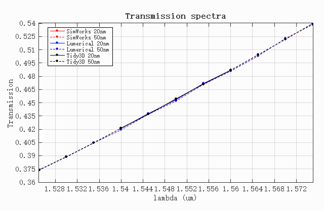
We start with the Staircase. In this case, the dielectric interfaces in all three software tools are approximated solely by the staircase of the Yee‑cell mesh. Therefore, this step can be used to verify the consistency of the three software tools in terms of basic settings such as geometric model, source excitation, and boundary conditions, providing a baseline for the subsequent comparisons. The figure below shows the transmission of the fundamental TE mode at the coupling port obtained with the three software tools. The results indicate that the deviation among the three software tools is less than 0.2%. This demonstrates that under a consistent mesh treatment, the results of the three software tools can mutually verify each other, and the deviation is within an acceptable range.

Results with a Polarized Subpixel Averaging Method at Material Boundaries #

The default treatment of material boundaries in all three software tools is to calculate an equivalent permittivity based on the mesh cells at the material interface, using the proportions of different materials and the relationship between the electric field and the normal direction of the structural surface (SimWorks: Conformal variant VP‑EP 0, Lumerical: conformal variant 0, Tidy3D: PolarizedAveraging). After adopting the respective default boundary treatment methods, the results are shown in the figure below. The coupling‑port transmissions of Lumerical and Tidy3D are very close, with a difference of less than 0.29%; the result of SimWorks is about 2% lower than the other two. This is because the default number of mesh refinement subcells in SimWorks is 5, which results in a lower boundary‑fitting accuracy for fine structures such as the directional coupler, leading to inaccurate computation of the gap width and consequently a lower coupling efficiency.

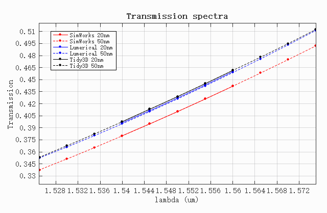
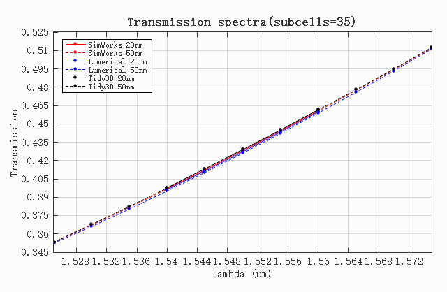
In SimWorks, apart from the staircase mesh, all other mesh refinement types include a setting for the number of mesh refinement subcells. This setting determines into how many subcells a single mesh cell is divided for the calculation of the equivalent permittivity. In a 2D simulation, a single mesh cell is divided into N×N subcells; in a 3D simulation, it is divided into N×N×N subcells, where N is the user‑specified mesh refinement subcell value. A larger number of subcells yields higher accuracy but also increases the computational cost; for special high‑precision requirements the number can be increased appropriately. The simulation result after increasing the number of mesh refinement subcells in SimWorks is shown in the figure below. When the number of subcells is 35, the maximum deviation from Tidy3D is only 0.102%, indicating that SimWorks can easily match the accuracy of the other software by adjusting this parameter.

For the typical silicon‑based directional coupler, the three software tools yield mutually verifiable simulation results under consistent basic settings, proving that their solver kernels are equivalent when the physical conditions are identical. Under the respective default conformal mesh settings, there are explainable quantitative differences among the three software results, which originate from the relatively conservative default value of the mesh refinement subcells in SimWorks. By increasing the number of mesh refinement subcells, the simulation results of SimWorks can be aligned with those of the other two software tools. In summary, the three software tools exhibit comparable precision at the core FDTD algorithm level, and their simulation results are all trustworthy.

References #

[1]Z. Liu and J. K. S. Poon, "Comparison of Lumerical FDTD and Tidy3D for three-dimensional FDTD simulations of passive silicon photonic components," Opt. Continuum, 4(10), 2427-2451 (2025).