Settings for TFSF Sources #

This section describes the settings for TFSF sources.

When studying scattering field problems, Total-Field Scattered-Field (TFSF) sources can be employed to directly acquire the scattering fields.

Select the TFSF in the solver tab and create a TFSF source in the Composite viewer, then set further parameters in the Edit properties interface that automatically pops up.

TFSF Sources #

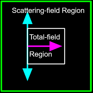
In FDTD, the TFSF source divides the calculation region into two distinct regions:

• Total field $\boldsymbol{E}_{total} = \boldsymbol{E}_{inc} + \boldsymbol{E}_{scat}$, i.e., the total field $\boldsymbol{E}_{total}$ is equal to the sum of the incident field $\boldsymbol{E}_{inc}$ and the scattering field $\boldsymbol{E}_{scat}$;
• The scattering-field region includes the scattering field $\boldsymbol{E}_{scat}$ only.

TFSF sources are often used to study scattering and antenna problems. Typical applications include:

• Particles in homogeneous media (which may be lossy or anisotropic), such as triple scattering;
• Aperiodic structures in multilayer substrates, which may be lossy or anisotropic;
• Periodic structures in multilayer substrates, when used with the periodic or Bloch boundary condition.

The option of TFSF source is an advanced feature. Users should determine the appropriate source settings according to these instructions to ensure accurate results. Otherwise, incorrect settings may lead to inaccurate results.

Settings for TFSF Sources #

General Settings #

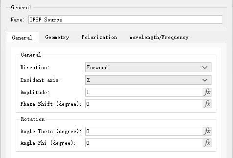
The General tab can be used to set the incident axis, amplitude, and other parameters related to a source.

Name	Description
Direction	The propagation direction of a TFSF source, specifically selected as Forward (forward propagation) or Backward (backward propagation).
Incident axis	Select the desired incident axis for a TFSF source from the drop-down list.
Amplitude	Source amplitude is set as 1 by default.
Phase shift	Used to set phase delay between multiple sources.
Angle theta	Polar angle. Angle between direction of source propagation and normal of incident plane.
Angle phi	Azimuthal angle. Angle between projection of source in propagation direction onto interface (if light propagates along Z-axis, XY plane represents interface) and positive X-axis.

By editing Angle theta and Angle phi in the General tab of the source, the injection angle of the source can be set. Note that Angle phi is only available in 3D simulations.

Geometry #

Gemetry tab can be used to set geometric dimensions of a source.

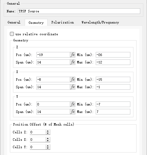
Name	Description
Use relative coordinate	Use relative coordinates.
Z/X/Y pos	Center of a source.
Z/X/Y span	Range of a source.
Cells Z/X/Y	Number of offset units in the Z/X/Y direction.

Polarization #

The Polarization tab can be used to set the polarization of a source. Linear polarization(θ) is the polarization angle for linear polarization.

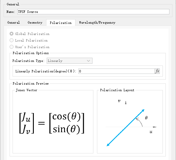
Wavelength/Frequency #

Wavelength/Frequency tab can be used to set wavelength/frequency of a source.

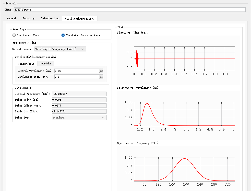
Name	Description
Continuous wave	Continuous wave.
Modulated gaussian wave	Modulated Gaussian wave.
Select domain	Select Wavelength or Time as the domain of input parameter.
Center/Span	Center/Span Used to set center wavelength and wavelength bandwidth.
Max/Min	Max/Min Used to set maximum and minimum values for bandwidth.
Central frequency	Define central wavelength.
Pulse width	Define pulse width which covers the wavelength or frequency range to be simulated.
Pulse offset	Defines pulse offset, i.e., time interval between start of the simulation and center of input pulse. Thus, the initial field is close to zero at the start of the simulation. To avoid interruption of the input pulse, the pulse offset should be at least twice the pulse duration to ensure that the frequency distribution is approximately symmetrical near the central frequency of the source.
Bandwidth	Define full width at half maximum (FWHM) of source in frequency domain.
Pulse type	Two types are available: Standard and Broadband. This is a read-only parameter.

Software provides wavelength/frequency domain images, which are plotted respectively for:

• Time domain signals;
• Wavelength domain spectrum;
• Frequency domain spectrum.

Notes for TFSF Sources #

Users should follow the guidelines below when using TFSF sources to avoid common errors in TFSF source settings and ensure the accuracy and reliability of simulation results.

Structural Settings for TFSF Sources #

When adding a TFSF source, ensure the following conditions:

• The scatterer must be completely located within the TFSF source;
• The wave vector of the source must be perpendicular to the substrate. In other words, all sides of the TFSF source must "see" the same refractive index distribution along the propagation direction.

Below are examples of valid and invalid settings:

Valid injection: The wave vector is perpendicular to the gold and glass layers. Each side of the source "sees" the same refractive index distribution (air-gold-glass) along the propagation direction (from the incident surface to the end surface).

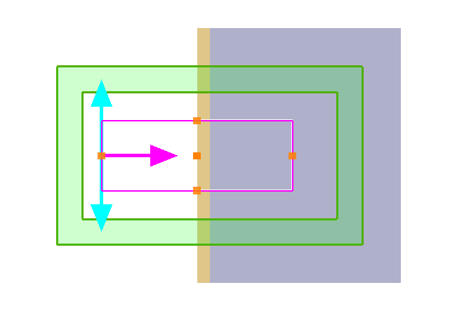
Invalid injection: The wave vector is not perpendicular to the substrate. The upper part of the source "sees" the refractive index of air, while the lower part "sees" the refractive index of the substrate.

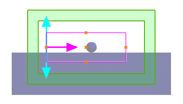
The internal structure of the TFSF source can be divided into two cases:

1. The TFSF source contains a single medium;
2. The TFSF source contains different media: currently, it is only applicable to scenarios where the propagation direction has a consistent medium distribution, such as multilayer materials. Complex distributions with different media inside the TFSF source are not yet supported.

The two cases are described in detail below:

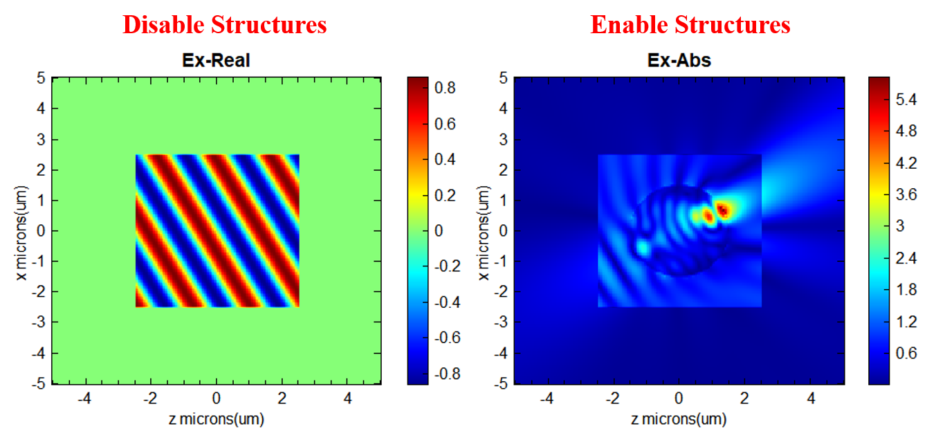
1. For a TFSF source containing only a single medium, the TFSF source supports arbitrary incidence angles.
It is recommended that users disable the material structure to check whether the TFSF source settings are correct before proceeding with oblique-incidence simulations. When the structure is disabled, the TFSF source propagates in vacuum and the electric field is concentrated only within the TFSF region (the total field), while the scattering field is nearly zero.

2. For multilayer material simulations, the normals of the material layers must be perpendicular to the TFSF injection plane. Under this configuration, oblique incidence is simulated by adjusting the source angle while keeping the material orientations fixed. Under this setting, fields transmitted through the substrate are strictly confined to the total-field region and cannot pass through the TFSF boundary into the scattering-field region. In the simulated multilayer $Si$-$SiO_2$ structure under oblique incidence below, complete absorption by the TFSF boundary ensures total isolation of the fields from the scattered-field region.

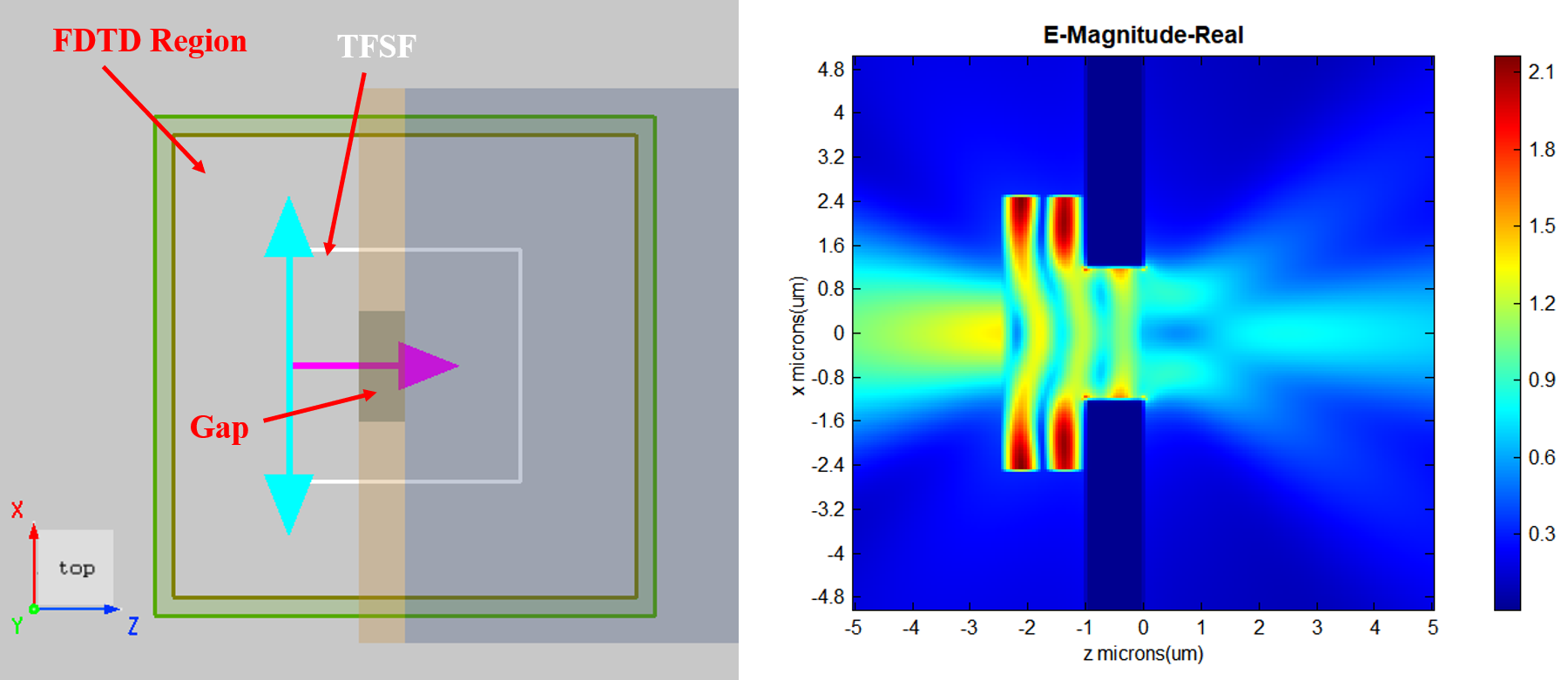
Additionally, in the air-gold-glass layer simulation shown above, introducing a gap within the gold layer allows scattered light to enter the scattered-field region. This gap acts as a scatterer and must be entirely contained within the interior of the TFSF source.

Currently, TFSF sources support non-uniform mesh simulations for all angles of incidence. If the simulation results are abnormal, it is recommended that users try switching to a uniform mesh for troubleshooting, in order to eliminate interference caused by mesh-related factors.

TFSF Sources Crossing Boundaries #

In general, TFSF sources should not cross the boundaries of the simulation region, with the following two exceptions:

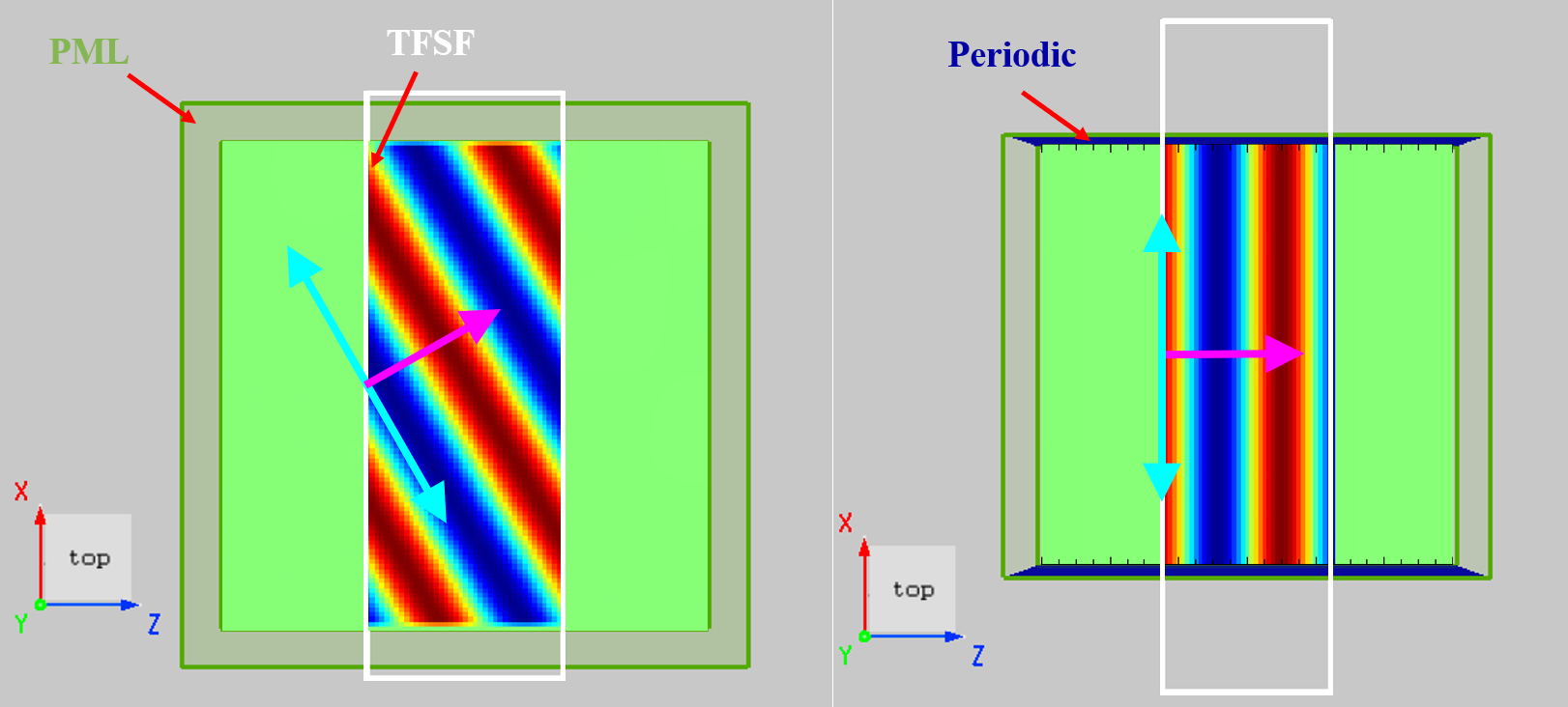
• At PML boundaries, the software will automatically constrain the source within the PML boundary, meaning the TFSF source is only effective inside the PML boundary.
• When using periodic boundaries, TFSF sources should cross the boundary. Also supports crossing Bloch boundaries.

Case: Mie Scattering #

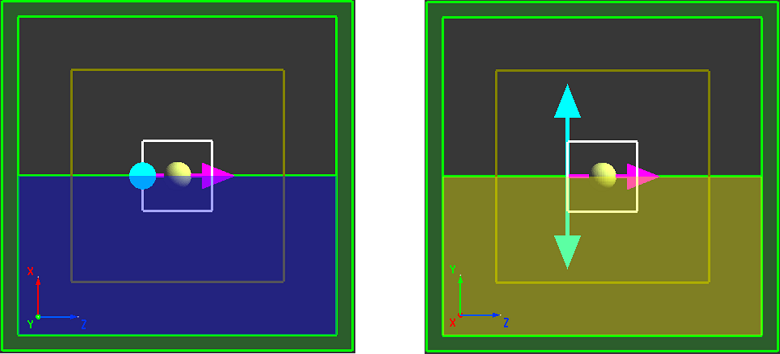
TFSF sources are used to study Mie scattering in this case. For related information, see Mie Scattering. The project is shown as below:

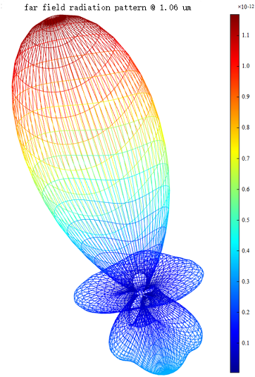
Once the simulation is completed, the scattered field (i.e., the field outside the space surrounded by the TFSF source) is extracted, and the far-field analysis is used to obtain the following polar plot and radiation pattern: