Common Control #

Data Import #

This section describes the import and export functions provided in the software.

Data Import #

You can import the following types of data on the interface:

• Formulas Import

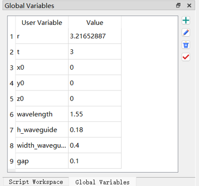
The software supports custom definitions of Global variables. On the Global tab, you can set the corresponding variables and values for specific projects.

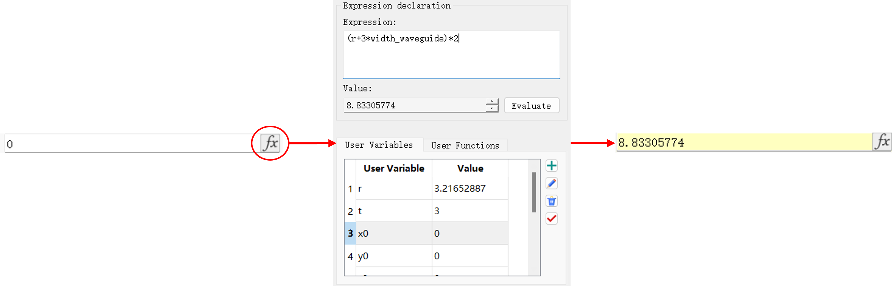
Click the $fx$, and enter the expression of the global variable. The result data of the expression will be returned on the software interface.

• Data Import

Then you can enter the data directly on this interface.

• Drop-down Menu

Select an item from the drop-down menu bar as an import.

• Activation

It is used to indicate whether a certain function is enabled or disabled in the project. The item will be enabled by clicking the checkbox to place a checkmark inside the box, or disabled by clicking the checkbox again to remove the checkmark.

• Options

The option button can be used to activate or deactivate an option. You can select only one option at a time from a set of option buttons. If one option is selected, the previously selected option will be automatically deactivated.

For formulas and data imports, the input data will be subject to restrictions based on the corresponding parameter domain.

Data Transfer #

There are diverse data types available in the software:

• Number
• String
• Matrix
• Struct
• Cell

For more information, see Data Types of scripts.

It should be particularly pointed out that the dataset is a data structure exclusive to the software. Please note that it is not a data type.

The dataset greatly simplifies the data management of the software. It not only enables creation, composition, modification, and import/export of simulation data, but also allows you to view data by using the Data Visualizer window.

The software supports data input and output through scripting:

• script import:

  • load_ascii("filename"): Import MaxCloud ascii data and load data in the .mdfascii format into the workspace;
  • loaddatafile: Load data in the .mdf format into the workspace;
  • loadmatlabmatfile: Import a dataset in the MATLAB's.mat format;
  • loadproject: Import project files.

• script export:

  • save_ascii: Save data as a.mdfascii file;
  • savedatafile: Save data as a.mdf file;
  • savematlabmatfile: Save data as a.mat file recognized by MATLAB;
  • saveproject: Save project files.

For more information on script import and export, see Script.

Unit Setting #

Defining basic physical units is a prerequisite for simulation. It is important to select proper physical units for different application scenarios. In the software ribbon, click File to display the application menu, users can set the physical units in Setting -> Physical units .

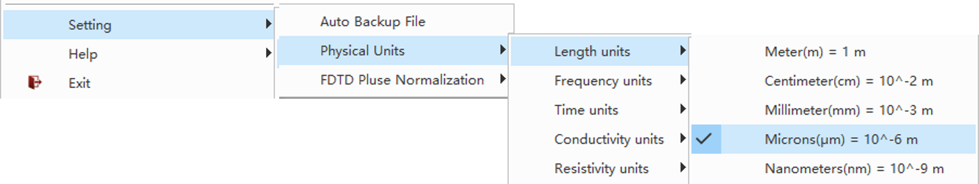
For more information, see Physical Quantities and Units.

Pulse Normalization #

Pulse Normalization Setting #

In the software ribbon, click File to display the application menu, users can select the desired normalization method in Setting->FDTD pulse normalization .

Name	Descriptions
No normalization	The result data to be returned is the Fourier transform of time-domain pulses.
Continuous wave normalization	Adjust the amplitude or power of pulse signals to a uniform scale.

In the FDTD solver, the FDFP monitor is used to record electric and magnetic fields within various frequency bands defined by the user. Selecting different normalization methods leads to different results to be returned. For example, the pulse signal $s(t)$ is:

$$s(t) = sin(\omega_0(t-t_0))exp(-\frac{(t-t_0)^2}{2(\Delta t)^2})$$

and the Fourier transform $s(\omega)$ of the time-domain pulse is:

$$s(\omega) = \int exp(-i\omega t)s(t)dt$$

The frequency-domain field $\boldsymbol{E}{sim}(\omega)$ under No normalization will be:

$$\boldsymbol{E}_{sim}(\omega) = \int exp(-i\omega t)\boldsymbol{E}(t)dt$$

If the Continuous wave normalization is applied, the frequency-domain field $\boldsymbol{E}_{imp}(\omega)$ will be subject to the normalization process using a frequency-domain pulse signal:

$$\boldsymbol{E}_{imp}(\omega) = \frac{\boldsymbol{E}_{sim}(\omega)}{s(\omega)}$$

Global Variables #

Scope of Global Variables #

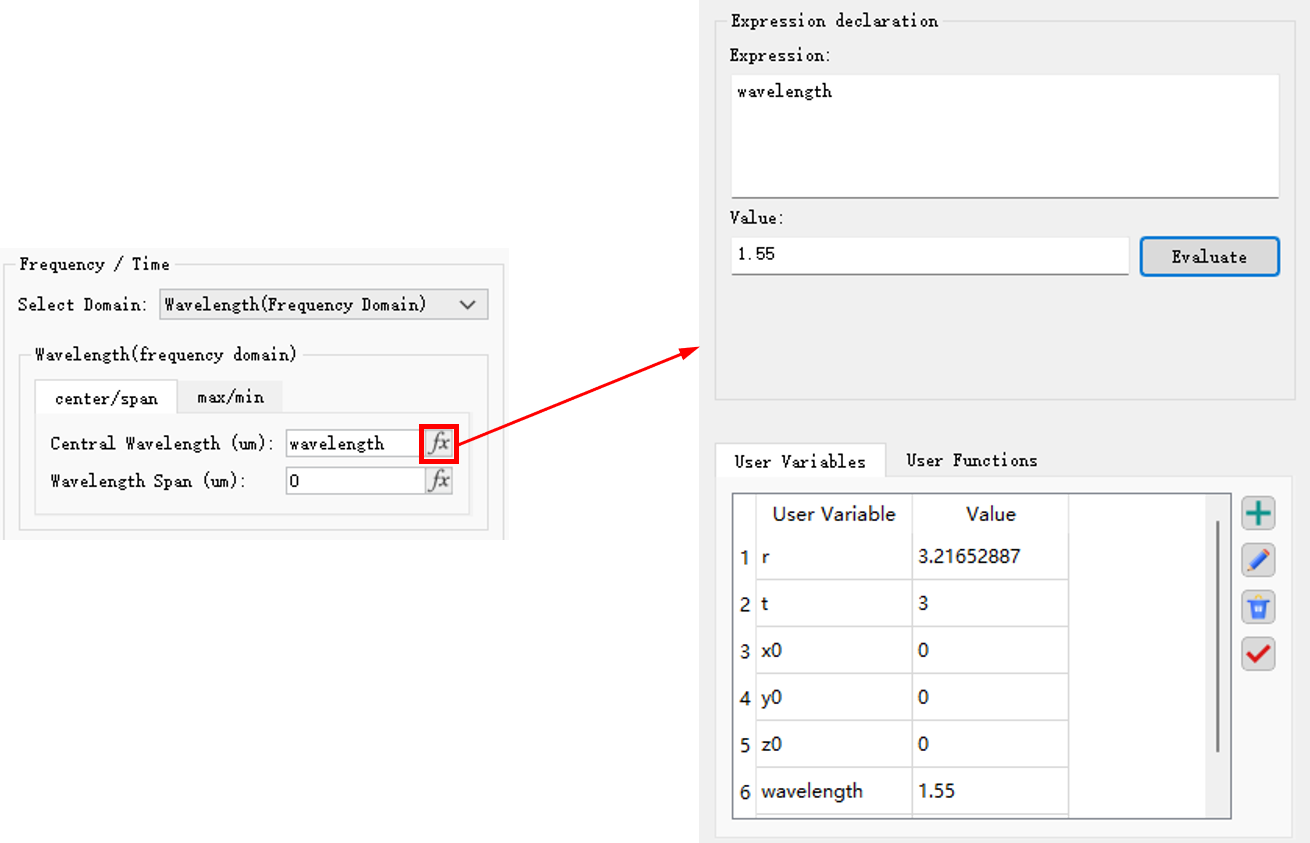
Global variables are primarily used for importing parameters into input boxes or scripts through expressions. They allow users to modify multiple interlinked parameters in a unified manner, realizing quick and efficient adjustment of simulation projects.
As shown in the figure below, users can directly enter the added global variables in the input box, or click the fx button to view and input the desired global variables in the pop-up page. It is important to note that global variables do not have units, and their physical unit is determined by the input.

In contrast to global variables, the software also offers local variables, such as variables in a script, whose scope is limited to the workspace of the script.

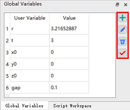
Define Global Variables #

Add global variables in the Global variables of the main interface. The four buttons on the right are used to manage global variables, with functions for "Add," "Edit," "Delete," and "Apply" respectively.

Coordinate System #

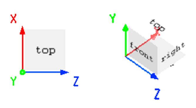
Cartesian Right-Hand Coordinate System #

When creating structures in the software, the Cartesian right-hand coordinate system is used.

• For 2D simulation, using the ZX plane;
• For 3D simulation, using the ZXY space.

Coordinate System Transformation #

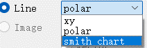
In the Data visualizer window, users can view Line-type images by switching over different coordinate systems to display the result. Currently, the software supports the following coordinate systems:

• xy
  Plot the relationship between one 1D vector and another. For multidimensional matrices, users can select a parameter in the Parameters list as the abscissa, and select a data in the Attributes list as the ordinate.

• Polar
  Plot the angular distribution of parameters. The data to be plotted should include radians and radial axes. The polar coordinates are expressed in degrees.

• Smith chart
  Plot impedance data.

Transmission Phase #

For transmission of time-domain pulse, two options are available:

• $exp(-i\omega t)$
• $exp(i\omega t)$

In this software, $exp(-i\omega t)$ represents a phase increase.

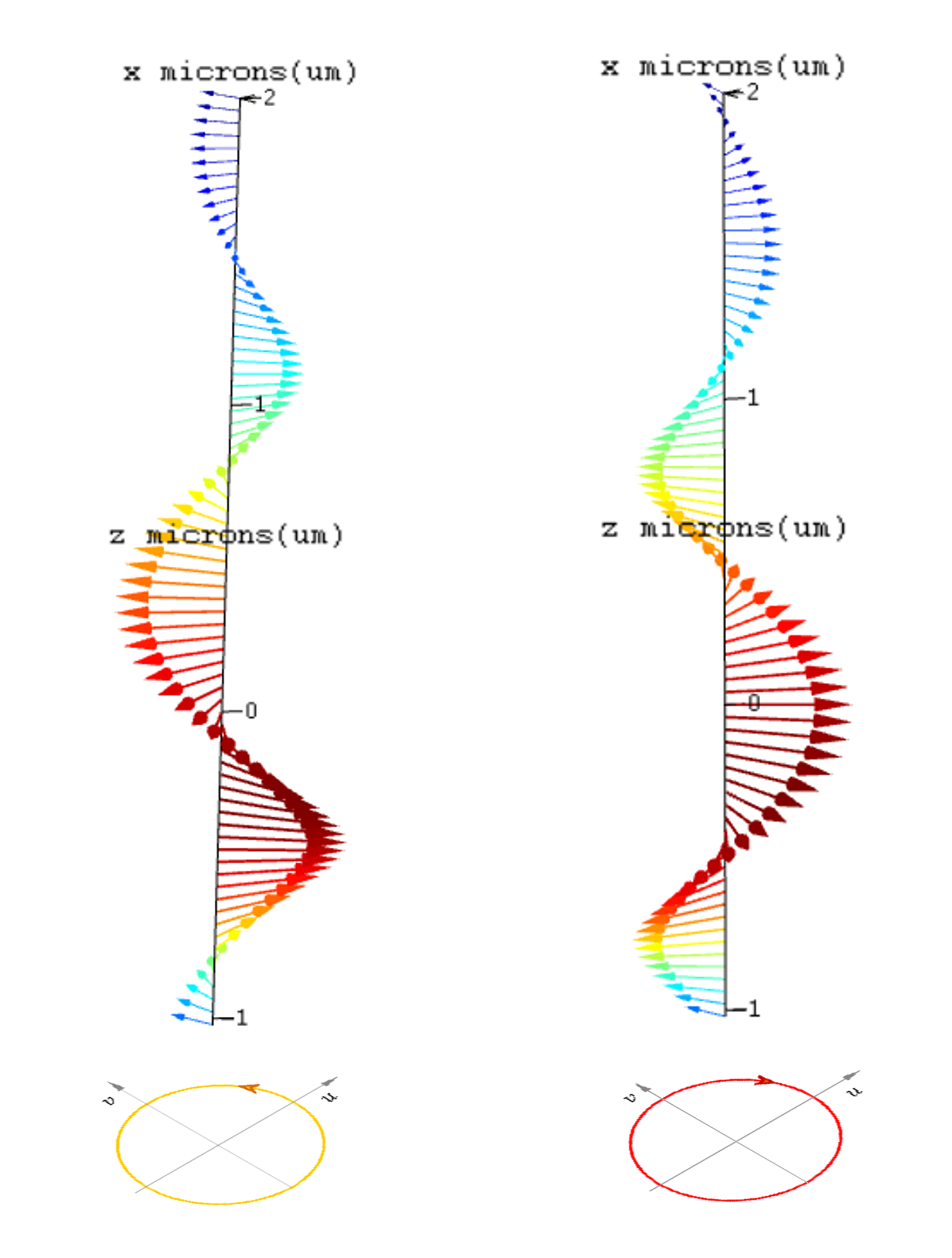
Circularly Polarized Light #

According to the rotation direction of the light vector, circularly polarized light can be divided into left-handed circularly polarized light and right-handed circularly polarized light.

• If the light vector rotates in the anti-clockwise direction (facing the direction of light propagation), it is left-handed circularly polarized light;
• If the light vector rotates in the clockwise direction (facing the direction of light propagation), it is right-handed circularly polarized light.

Circularly polarized light can be regarded as the synthesis of two plane-polarized lights with same frequency and amplitude, that have the orthogonality in their vibration directions, and a phase difference of $± π/2$. Wherein, the phase difference of $+π/2$ and $-π/2$ corresponds to left-handed circularly polarized light and right-handed circularly polarized light respectively.

As shown in the figure below, the left side is the vector diagram of left-handed polarized light, and the right side is the vector diagram of right-handed circularly polarized light.