Preface #

Fiber Bragg Grating (FBG) is an optical filtering device formed by introducing a periodic refractive index modulation in the fiber core, widely used in optical fiber communications, fiber sensing, laser frequency stabilization, and other fields. When light propagates through the fiber, the FBG selectively reflects a specific wavelength that satisfies the Bragg condition, while transmitting all other wavelengths, making it an efficient optical filter. In this example, the Eigenmode Expansion (EME) solver is employed to simulate the fiber Bragg grating. Through conventional parameter sweep and wavelength sweep, the computational efficiency advantage of EME in handling long-period grating structures is demonstrated.

Simulation settings #

Structure Description #

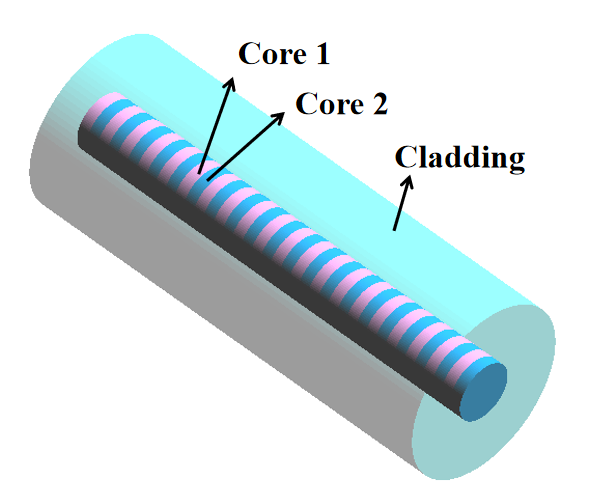
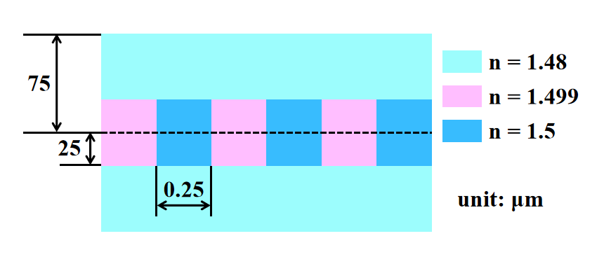
As shown in the figure, the FBG has a ring-shaped fiber core structure. The cladding region is a circular ring with an outer radius of $75\ \text{μm}$ and an inner radius of $25\ \text{μm}$, with a refractive index of $1.48$. The fiber core is located inside the cladding and consists of two different materials arranged alternately along the fiber axis as cylinders. The cylinders all have a radius of $25\ \text{μm}$ and a thickness of $0.25\ \text{μm}$, with refractive indices of $1.499$ and $1.5$, respectively. Two adjacent cylinders together form a basic periodic unit.

Solver Settings #

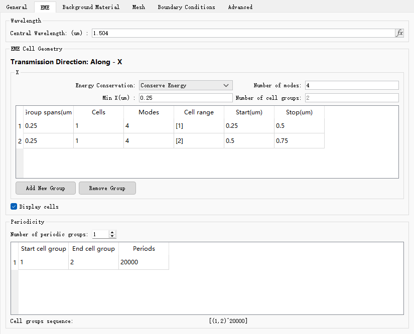
Add an EME solver such that it covers one basic periodic unit of the fiber Bragg grating. Set up a port at each end of the solver region to calculate the transmission and reflection into the fundamental mode. In the EME setup tab, define two cell groups, one covering the high‑index region and the other covering the low‑index region. To set the periodicity of the FBG, define a periodic group under Periodicity. Set the Start cell group and End cell group to $1$ and $2$, respectively, and set Periods to $20000$. This means that one basic periodic unit is repeated 20,000 times, making the total length of the FBG $1\ \text{cm}$.

仿真结果 #

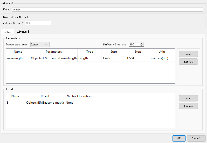
EME is a frequency‑domain method; to obtain a full transmission or reflection spectrum, multiple wavelengths must be simulated individually. Therefore, the parameter sweep function is used. Open the attached simulation project Fiber_Bragg_gratings.mpps, which contains a pre‑configured parameter sweep with 100 points, sweeping the center wavelength from $1.495\ \text{µm}$ to $1.504\ \text{µm}$. The sweep results are stored in the user s‑matrix. Right‑click on the sweep you wish to run and select Run. After the sweep finishes, you can run the plot_parameter_sweep.msf script to plot the transmission spectrum of the FBG, as shown in the figure. To increase the spectral resolution, simply increase the number of sweep points. It should be noted that because the parameter sweep recalculates the mode field at each wavelength and performs a full simulation, the computational cost increases with the number of points. If the mode field does not change significantly with wavelength, you can use the EME wavelength sweep feature for a fast estimation.

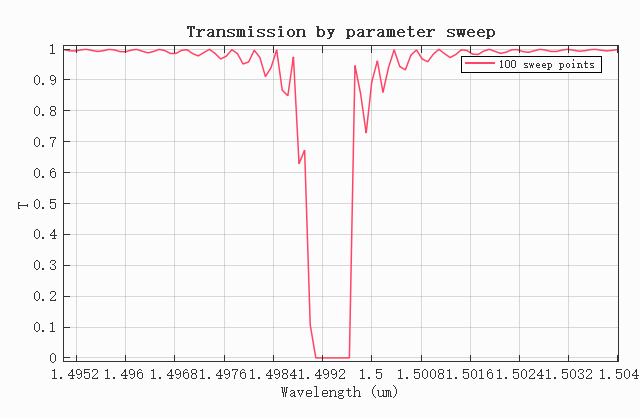
The wavelength sweep feature of EME does not recompute the modes; instead, it obtains the wavelength dependence of the S‑matrix by simply varying the wavelength. This is useful for quickly estimating the device response during the early design phase. Click the To Run button to run the simulation, then enable Wavelength sweep in the EME Analysis Window .Set the Start wavelength to $1.495\ \text{µm}$ and the Stop wavelength to $1.504\ \text{µm}$, set the Number of wavelength points to $100$, and click the Wavelength sweep button. After the wavelength sweep finishes, run the parameter_sweep_vs_wavelength_sweep.msf script to plot the results of both sweeps on the same graph. It can be seen that the results from the wavelength sweep and the parameter sweep are essentially identical.

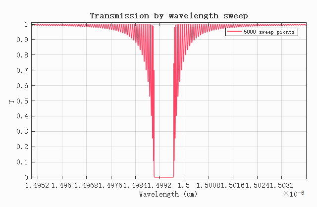
To obtain a higher‑resolution transmission spectrum, set the number of sweep points to 5000; the result is shown below, taking only a few seconds.

The EME solver is specifically designed for planar waveguide structures. Based on mode‑coupling theory, it efficiently decomposes any arbitrary input field into a linear combination of eigenmodes of the waveguide cross‑section and solves Maxwell's equations in the frequency domain with boundary conditions. This approach accurately computes mode coupling and evolution while significantly improving computational efficiency without sacrificing accuracy. It has become the preferred tool for simulating the transmission characteristics of complex waveguide systems in the development of integrated optical devices.