Settings for Dipole Sources #

This section describes settings for dipole sources.

In FDTD, an electric dipole generates a field around the oscillating point charge, while a magnetic dipole exhibits field distribution around a current loop.

Select Dipole in the solver tab and create a dipole in the Composite viewer, then set further parameters in the Edit properties interface that automatically pops up.

Ideal Dipole Field #

In FDTD, a Dipole acts as source $\rho$ for generating the electromagnetic field in Maxwell's equations.

Typical electric and magnetic dipoles are shown in the figure below:

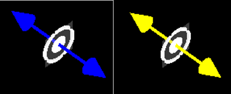
The Monopole, Dipole, Quadrupole, Hexapole, and Octupole can't be accomplished by a simple superposition of dipoles because polarization intensity, $p$ in this case, involves a complex polarization tensor that cannot be described by a superposition of dipoles.

Dipole Settings #

General Settings #

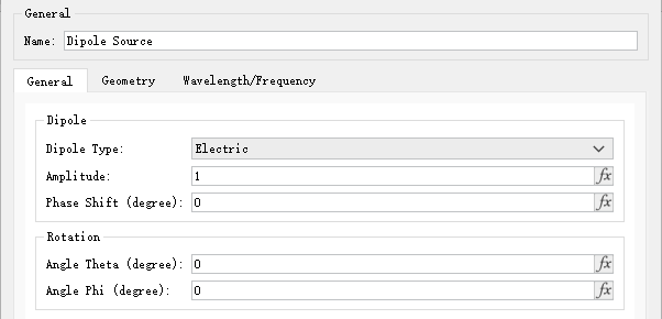
The General tab is used to set the properties of the dipole. The Dipole Type option selects the type of dipole, as detailed below:

Name	Descriptions
Electric	Electric dipole.
Magnetic	Magnetic dipole.

Name	Description
Amplitude	Source amplitude is set as 1 by default.
Phase shift	Used to set phase delay between multiple sources.
Angle theta	Polar angle. Angle between direction of source propagation and normal of incident plane.
Angle phi	Azimuthal angle. Angle between projection of source in propagation direction onto interface (if light propagates along Z-axis, XY plane represents interface) and positive X-axis.

By editing Angle theta and Angle phi in the General tab of the source, the injection angle of the source can be set. Note that Angle phi is only available in 3D simulations. For a dipole source, Angle theta represents the angle between the dipole vector and the Z axis, and Angle phi is the angle between the projection of the dipole vector onto the XY plane and the positive X direction.

Geometry #

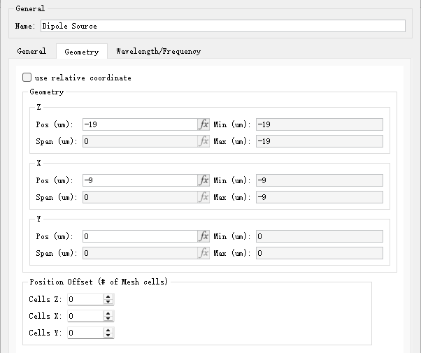
Gemetry tab can be used to set geometric dimensions of a source.

Name	Description
Use relative coordinate	Use relative coordinates.
Z/X/Y pos	Center of a source.
Z/X/Y span	Range of a source.
Cells Z/X/Y	Number of offset units in the Z/X/Y direction.

Wavelength/Frequency #

Wavelength/Frequency tab can be used to set wavelength/frequency of a source.

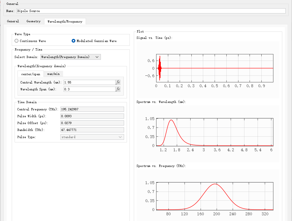
Name	Description
Continuous wave	Continuous wave.
Modulated gaussian wave	Modulated Gaussian wave.
Select domain	Select Wavelength or Time as the domain of input parameter.
Center/Span	Center/Span Used to set center wavelength and wavelength bandwidth.
Max/Min	Max/Min Used to set maximum and minimum values for bandwidth.
Central frequency	Define central wavelength.
Pulse width	Define pulse width which covers the wavelength or frequency range to be simulated.
Pulse offset	Defines pulse offset, i.e., time interval between start of the simulation and center of input pulse. Thus, the initial field is close to zero at the start of the simulation. To avoid interruption of the input pulse, the pulse offset should be at least twice the pulse duration to ensure that the frequency distribution is approximately symmetrical near the central frequency of the source.
Bandwidth	Define full width at half maximum (FWHM) of source in frequency domain.
Pulse type	Two types are available: Standard and Broadband. This is a read-only parameter.

Software provides wavelength/frequency domain images, which are plotted respectively for:

• Time domain signals;
• Wavelength domain spectrum;
• Frequency domain spectrum.

Advanced #

• You can add a Dipole Cloud analysis group in Analysis library to generate a specified number of dipoles, where the position, phase, and direction of each dipole are randomly distributed;
• Non-mesh dipoles can be formed by allocating the data of dipoles on nearby mesh points to the non-mesh dipoles based on distance;
• When simulating non-polarized dipoles, three dipoles with mutual orthogonality must be simulated three times.

Case: Bandstructure of 3D Cubic Lattice #

In this case, a randomly excited Dipole source is used to calculate the bandgap of a photonic crystal. For details, see Bandstructure of 3D Cubic Lattice.