通用控制 #

数据的输入 #

本节是关于软件中数据输入的介绍

数据输入 #

界面输入有以下几种类型：

• 公式输入

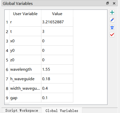
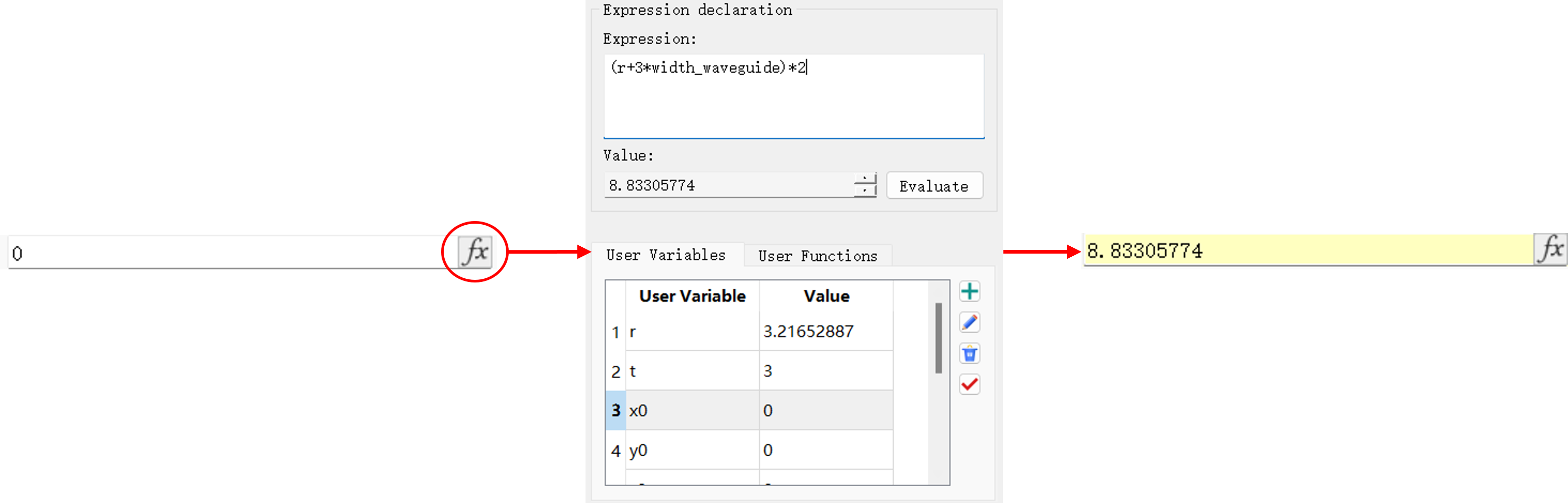
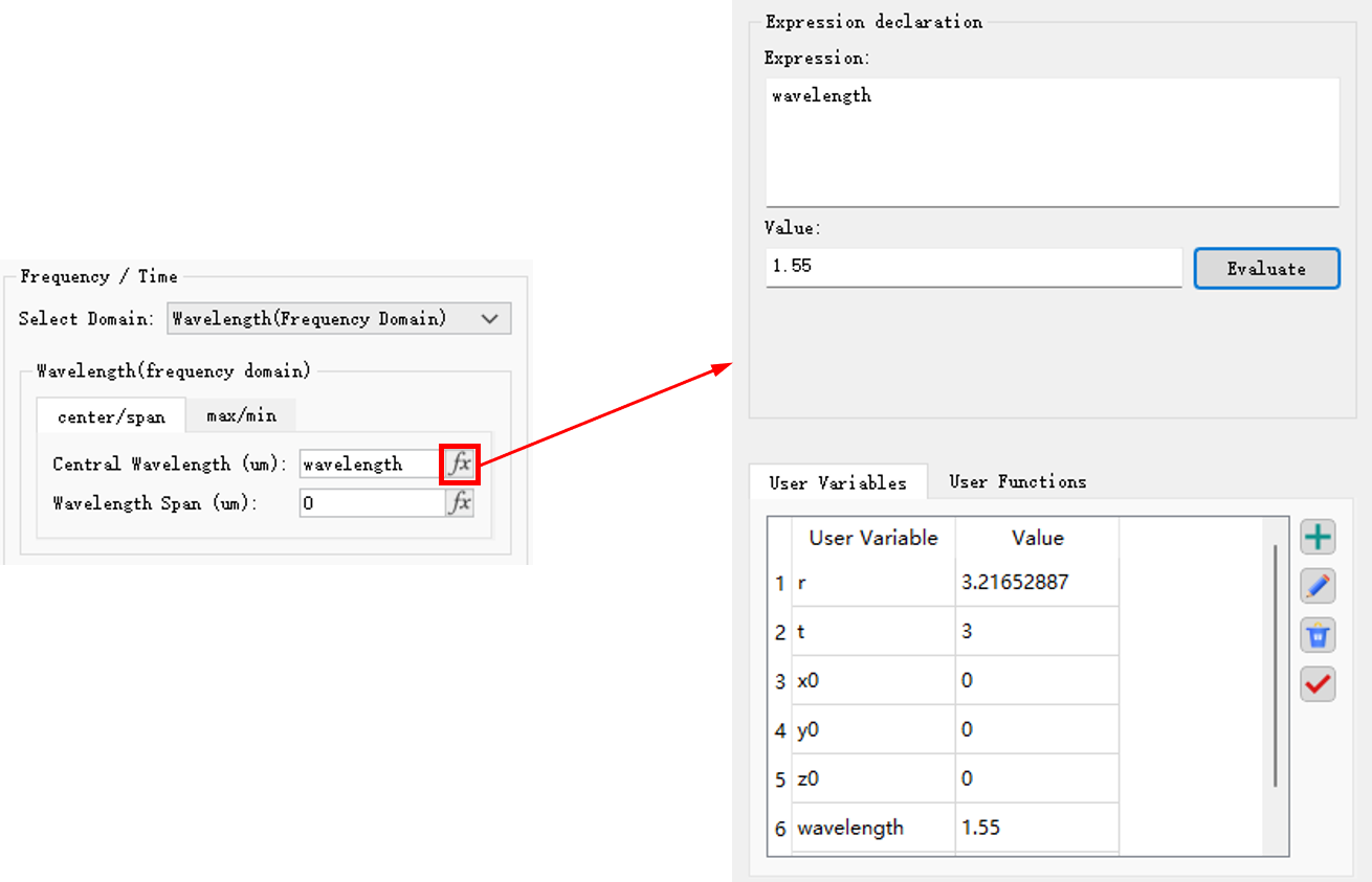
软件支持定义全局变量，在Global variables标签页，结合工程设置相应变量和值。

点击$fx$，输入全局变量的表达式，软件界面返回表达式的结果数据。

• 数据输入

在软件界面直接输入数据。

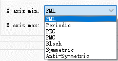
• 下拉菜单

从下拉菜单栏中选择项目作为输入。

• 激活

用于表示工程中启用或禁用某些功能。勾选表示启用该项，未勾选表示禁用该项。

• 选项

可以打开或关闭的选项按钮。在一组选项按钮中，用户一次只能选中一个选项，如果用户选择另一个选项，则先前选择的选项会被取消。

在公式输入和数据输入过程中，所输入的数据均受到相应参数定义域的限制。

数据传递 #

软件存在多种数据类型：

• Number
• String
• Matrix
• Struct
• Cell

相关介绍请参阅脚本的数据类型部分。

特别强调的是，数据集是软件独有的数据结构，请注意，此处不是数据类型。

数据集具备仿真数据的创建、组成、修改、导入/导出，以及通过数据可视化窗口查看数据等功能，极大地便利了软件数据的管理。

软件还支持脚本进行数据的输入和输出：

• 脚本输入：

  • load_ascii("filename")输入 MaxCloud ascii 数据，将.mdfascii格式的数据加载到工作区；
  • loaddatafile将.mdf格式的数据加载到工作区；
  • loadmatlabmatfile 输入 MATLAB 的.mat格式的数据集；
  • loadproject输入工程文件。

• 脚本输出：

  • save_ascii将数据保存为.mdfascii文件；
  • savedatafile将数据保存为.mdf文件；
  • savematlabmatfile将数据保存为 MATLAB 可识别的.mat文件；
  • saveproject保存工程文件。

有关脚本输入和输出的详细介绍请参阅Script。

单位设置 #

仿真的前提是做好对基本物理单位的规定，对于不同的应用情景，需要选择恰当的物理量单位。在软件功能区，用户可以点击 File 显示应用程序菜单，在Setting -> Physical units中设置物理量单位。

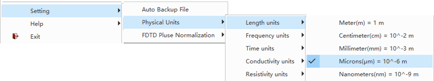
详情请参阅物理量和单位。

脉冲归一 #

脉冲归一的设置 #

在软件功能区中，点击 File 显示应用程序菜单，在Setting -> FDTD pulse normalization中选择归一化的方式。

Name	Descriptions
No normalization	非归一化；返回的结果数据是时域脉冲的傅里叶变换。
Continuous wave normalization	连续波归一化；将脉冲信号的振幅或功率调整为统一的尺度。

在FDTD求解器中，FDFP监视器记录一系列用户自定义频段下的电场和磁场。选择不同的归一化方式返回的结果数据不同。比如：时域脉冲信号$s(t)$为：

$$s(t) = sin(\omega_0(t-t_0))exp(-\frac{(t-t_0)^2}{2(\Delta t)^2})$$

时域脉冲的傅里叶变换$s(\omega)$为：

$$s(\omega) = \int exp(-i\omega t)s(t)dt$$

对于非归一化的频域场$\boldsymbol{E}_{sim}(\omega)$为：

$$\boldsymbol{E}_{sim}(\omega) = \int exp(-i\omega t)\boldsymbol{E}(t)dt$$

对于连续波归一化的频域场$\boldsymbol{E}_{imp}(\omega)$，需要使用频域脉冲信号归一化处理，为：

$$\boldsymbol{E}_{imp}(\omega) = \frac{\boldsymbol{E}_{sim}(\omega)}{s(\omega)}$$

全局变量 #

全局变量的作用域 #

用户在使用表达式输入参数时，可通过全局变量统一调整相互关联的参数，实现快捷、高效地调整仿真工程。
如下图所示，用户可以在对应输入框中直接输入已添加的全局变量，也可以点击fx按钮，在弹出页面中查看并输入所需的全局变量。需要注意的是，全局变量没有单位，其物理量单位由对应输入项决定。

与全局变量相对的是局部变量，例如脚本中的变量，作用域仅限在脚本的工作空间。

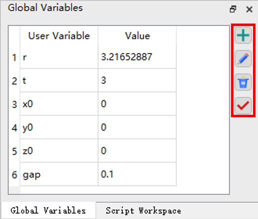
定义全局变量 #

在主界面的全局变量组件中，添加全局变量。右侧四个按钮用于管理全局变量，分别为“添加”，“编辑”，“删除”，“应用”。

坐标系 #

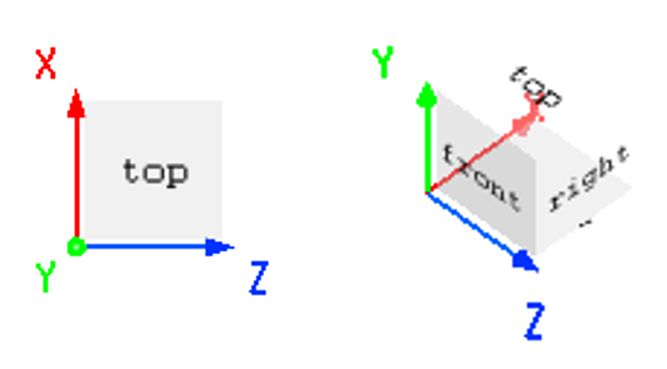
笛卡尔右手坐标系 #

软件创建结构时，使用笛卡尔右手坐标系。

• 二维仿真，使用 ZX 平面；
• 三维仿真，使用 ZXY 空间。

坐标系变换 #

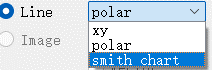
在可视化窗口中，对于Line类型的图像，用户可以切换不同的坐标系查看结果图像，目前软件支持的坐标系有：

• xy
  用于绘制一个 1D 向量与另一个 1D 向量的关系。对于大于 1 维的矩阵，用户可在Parameters列表选择一个参数作为横坐标，在Attributes列表中选择一个数据作为纵坐标。

• Polar
  极坐标图可以绘制参数的角度分布。绘制的数据需包括弧度和径轴，极坐标的单位是度。

• Smith chart
  史密斯图可以绘制阻抗数据。

传输相位 #

对于时域光信号的传输，有：

• $exp(-i\omega t)$
• $exp(i\omega t)$

本软件中，$exp(-i\omega t)$作为相位增加。

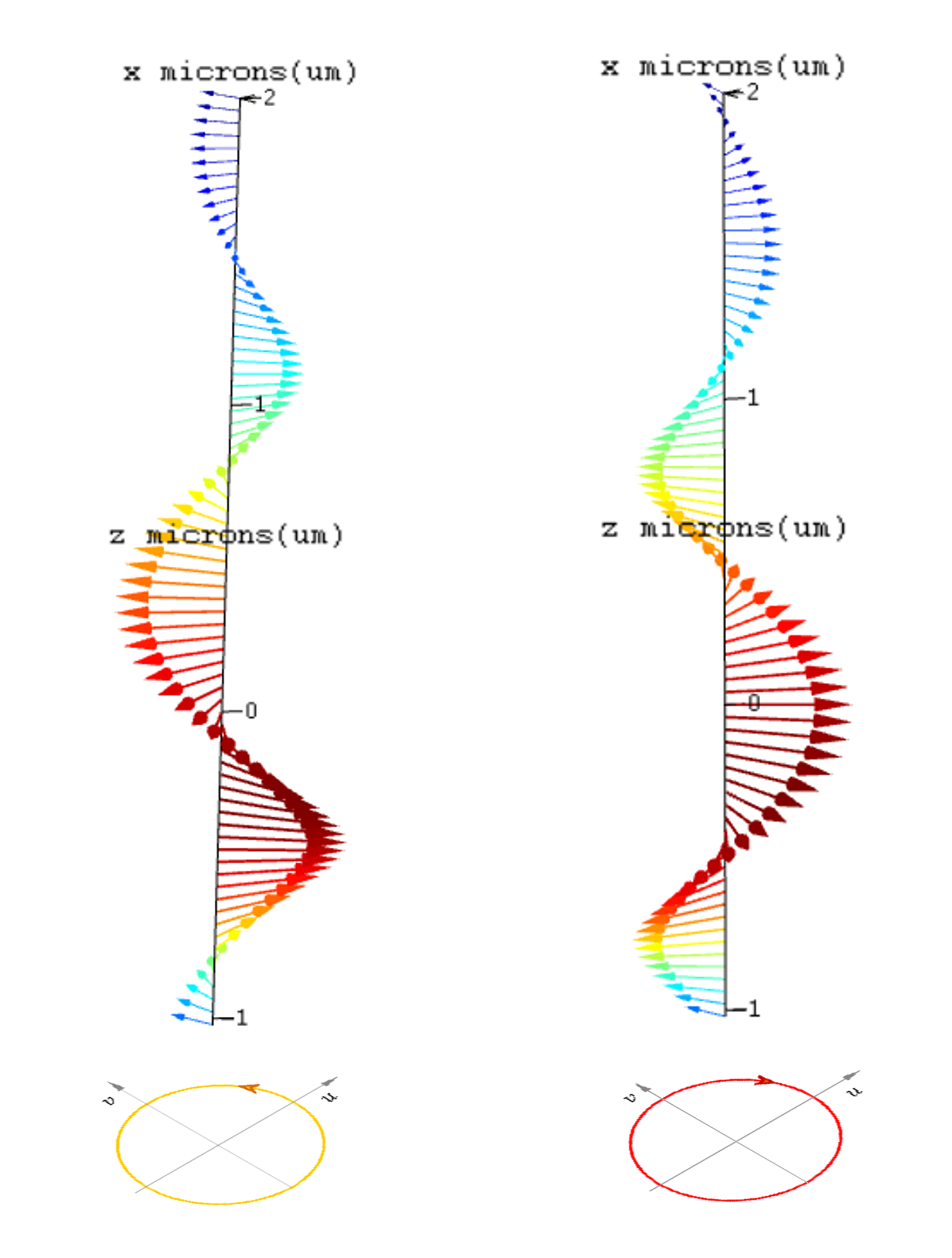
圆偏振光 #

根据光矢量旋转方向的不同，圆偏振光分为左旋圆偏振光和右旋圆偏振光。

• 迎着光传播方向观察，若光矢量沿着逆时针方向旋转，则为左旋圆偏振光；
• 迎着光传播方向观察，若光矢量沿着顺时针方向旋转，则为右旋圆偏振光。

圆偏振光可以看作是振幅相等、振动方向正交、相位差为$± π/2$的两个同频率的平面偏振光的合成。其中相位差为 $+π/2$ 时为左旋圆偏振光，相位差为 $-π/2$ 时为右旋圆偏振光。

如下图所示左侧为左旋偏振光的矢量图，右侧为右旋圆偏振光矢量图。