Y 分束器的逆向设计

时域有限差分(FDTD)光波导耦合器/分束器

2025-12-30 09:52:51

前言

近年来，逆向设计（inverse design）已经成为光子器件开发中的重要方法论。相比传统依赖经验、直觉或大量参数扫描的正向设计流程，逆向设计将器件开发重新表述为一个具有明确性能指标的优化问题。通过设定期望的电磁响应，并允许算法在设计空间中自由搜索，逆向设计能够自动生成许多难以通过人工经验推导的高性能光子结构。

在本案例中，我们以一个 Y 分束器作为示例，如何通过参数化结构描述实现器件几何的自动优化。通过算法自动调整参数化几何的控制点，使设计过程更加高效，器件性能更加卓越。

仿真设置

本案例中的完整仿真流程由附件中的 Python 脚本 simworks_ybranch_opt3D.py 自动驱动，无需人工在软件界面中设置结构或光源。脚本基于 SimWorks 的逆向设计优化框架构建，有关该优化框架的完整理论说明与接口使用方法，可参考用户手册中的逆设计介绍。

完整代码包含以下核心模块：

基础环境配置

脚本首先配置软件接口路径，并导入必要的 python 科学计算库（如 NumPy、SciPy）。其中， os.add_dll_directory 及 sys.path.append 的路径需分别指向软件安装目录下的 \bin 和 \api\python 文件夹。
```
import os
import sys

# This is the default installation path. If you install the software in a different directory, please update the path accordingly.
os.add_dll_directory(r"C:\Program Files\SimWorks\SimWorks FD Solutions\bin")
sys.path.append(r"C:\Program Files\SimWorks\SimWorks FD Solutions\api\python")

import numpy as np
import scipy as sp
import simworks
from debug_simworksybranch import simwork_ybranch_init
```
所需依赖库可以通过以下命令一键安装，若遇问题，请参考各库的官方文档（NumPy、SciPy、Matplotlib、PyQt6）。
```
pip install numpy scipy matplotlib PyQt6
```
随后，脚本通过调用 simwork_ybranch_init 函数加载预定义的基础仿真模型文件debug_simworksybranch.py。该模型定义了SOI平台的完整仿真环境，以及优化必须包括的对象，包括： $1.3-1.8\ \mu m$ 的宽带模式光源source，形状优化的FDFP监视器（opt_fields）, 输出端功率监视器(fom), 自定义网格(Mesh)。

参数化几何建模

逆向设计的核心在于将连续的物理结构转化为一组离散的、可优化的参数。本案例采用 “控制点+样条插值” 的参数化策略：在器件的分束区域定义 $20$ 个控制点的多边形结构，其 $X$ 坐标固定并均匀分布，而 $Y$ 坐标则作为待优化的变量。

# Define the span and number of points
initial_points_x = np.linspace(-1.0e-6, 1.0e-6, 10)
initial_points_y = np.linspace(0.25e-6, 0.6e-6, initial_points_x.size)


def splitter(params):
    ''' Defines a taper where the paramaters are the y coordinates of the nodes of a cubic spline. '''

    ## Include two set points based on the initial guess. The should attach the optimizeable geometry to the input and output 
    points_x = np.concatenate(
        ([initial_points_x.min() - 0.01e-6], initial_points_x, [initial_points_x.max() + 0.01e-6]))
    points_y = np.concatenate(([initial_points_y.min()], params, [initial_points_y.max()]))

    ## Up sample the polygon points for a smoother curve. Some care should be taken with interp1d object. Higher degree fit
    # "cubic", and "quadratic" can vary outside of the footprint of the optimization. The parameters are bounded, but the
    # interpolation points are not. This can be particularly problematic around the set points.
    n_interpolation_points = 20
    polygon_points_x = np.linspace(min(points_x), max(points_x), n_interpolation_points)
    interpolator = sp.interpolate.interp1d(points_x, points_y, kind='cubic')
    polygon_points_y = interpolator(polygon_points_x)

    ### Zip coordinates into a list of tuples, reflect and reorder. Need to be passed ordered in a CCW sense 
    polygon_points_up = [(x, y) for x, y in zip(polygon_points_x, polygon_points_y)]
    polygon_points_down = [(x, -y) for x, y in zip(polygon_points_x, polygon_points_y)]
    polygon_points = np.array(polygon_points_up[::-1] + polygon_points_down)
return polygon_points

在每一次优化迭代中，算法会根据当前这组 Y 坐标值，通过三次样条插值生成一条光滑、连续的边界曲线。此曲线经镜像对称后，即构成分束器的完整多边形几何轮廓。

InverseofYBranch_structure

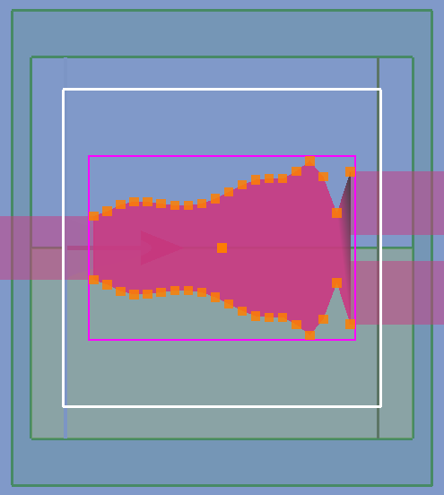
为确保最终结构的可制造性，每个控制点的 $Y$ 坐标被约束在 $0.2$ 至 $0.8\ \mu m$ 的物理范围内。这种参数化方法在设计自由度（通过控制点数量调节）与优化计算效率之间取得了良好平衡。

优化问题构建

我们定义了明确的优化目标：最大化光从输入端到输出端的总透射效率。在脚本中，这一目标通过 ModeMatch 模块实现，其理想目标值被设定为在全波段透射率均为 1。
```
######## FIGURE OF MERIT ########
fom = ModeMatch(monitor_name='fom',
                mode_number='fundamental mode',
                direction='Forward',
                target_T_fwd=lambda wl: np.ones(wl.size),
                norm_p=1)

######## OPTIMIZATION ALGORITHM ########
scaling_factor = 1.0e6
optimizer = ScipyOptimizers(max_iter=30,
                            method='L-BFGS-B',
                            scaling_factor=scaling_factor,
                            pgtol=1.0e-5,
                            ftol=1.0e-5,
                            scale_initial_gradient_to=0.0)
```
优化算法选用高效的 L-BFGS-B（拟牛顿法），最大迭代次数设为 30。为实现快速梯度计算，脚本启用了伴随法（Adjoint Method）。该方法仅需两次电磁仿真（一次正向、一次伴随）即可计算出目标函数对所有控制点参数的梯度，将计算复杂度从传统扰动法的 O(N) 降至 O(1)，极大地加速了优化进程。
自动化优化控制

集成上述模块后，脚本启动一个全自动的优化闭环，其流程如下：
1. 几何更新：基于当前控制点参数生成新的多边形边界
2. 电磁仿真：自动调用SIMWORKS进行FDTD计算
3. 性能评估：计算输出端透射率与目标值的差异
4. 梯度计算：通过伴随法计算目标函数对每个控制点的梯度
5. 参数更新：优化器根据梯度信息更新控制点位置
该循环持续进行直至收敛或达到最大迭代次数。整个过程完全自动化，无需人工干预。

仿真结果

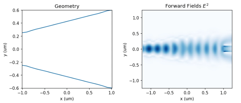
在展示最终优化结果之前，我们首先给出迭代过程中的中间结果，以便观察结构与性能的收敛趋势。下图展示了第 1 次迭代时分束区域的器件形状以及光场传播分布。可以看到，此时结构的总透射率较低，能量在分束过渡区域出现明显辐射损耗。

Iteration1

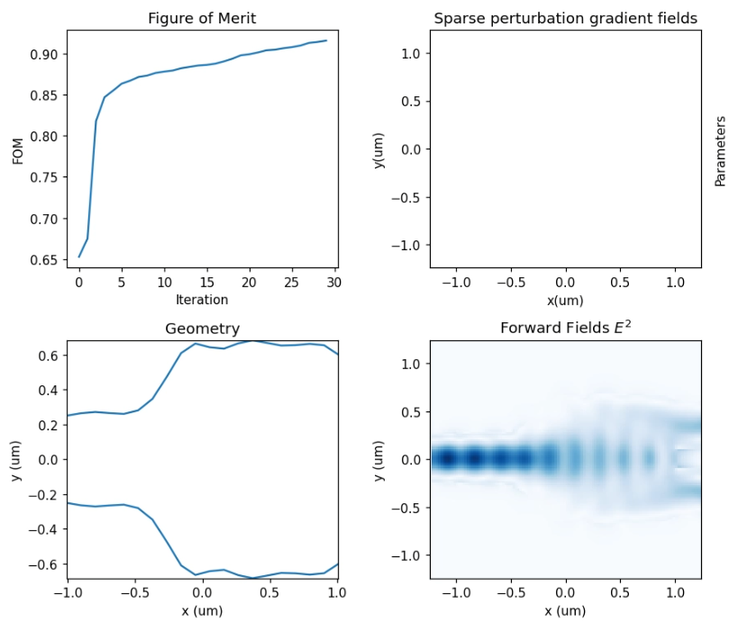
随着优化迭代的推进，分束区的几何逐渐被调优，光场过渡显著变得更加平滑。优化结束后，程序会自动生成并保存最终的三维工程文件，以及两个优化过程记录文件。其中 optimization_report.txt 记录了每一代的FOM值与优化的参数，convergence_report.txt 则保存了完整的迭代历史数据用于收敛分析。

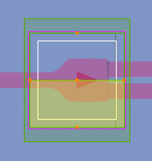
最终生成的三维工程文件如下图所示，可直接在SimWorks软件中打开进行后续分析：

final_simulation