FDE仿真控制面板
FDE仿真控制面板 #
本节是关于本征模有限差分(FDE)仿真控制平台设置的介绍。
添加FDE求解器并设置完工程后,点击FDE选项卡的To run按钮以运行软件,软件右侧界面会自动弹出仿真控制面板,模式分析被设置在仿真控制平台内。
仿真控制界面 #
模式分析窗口 #
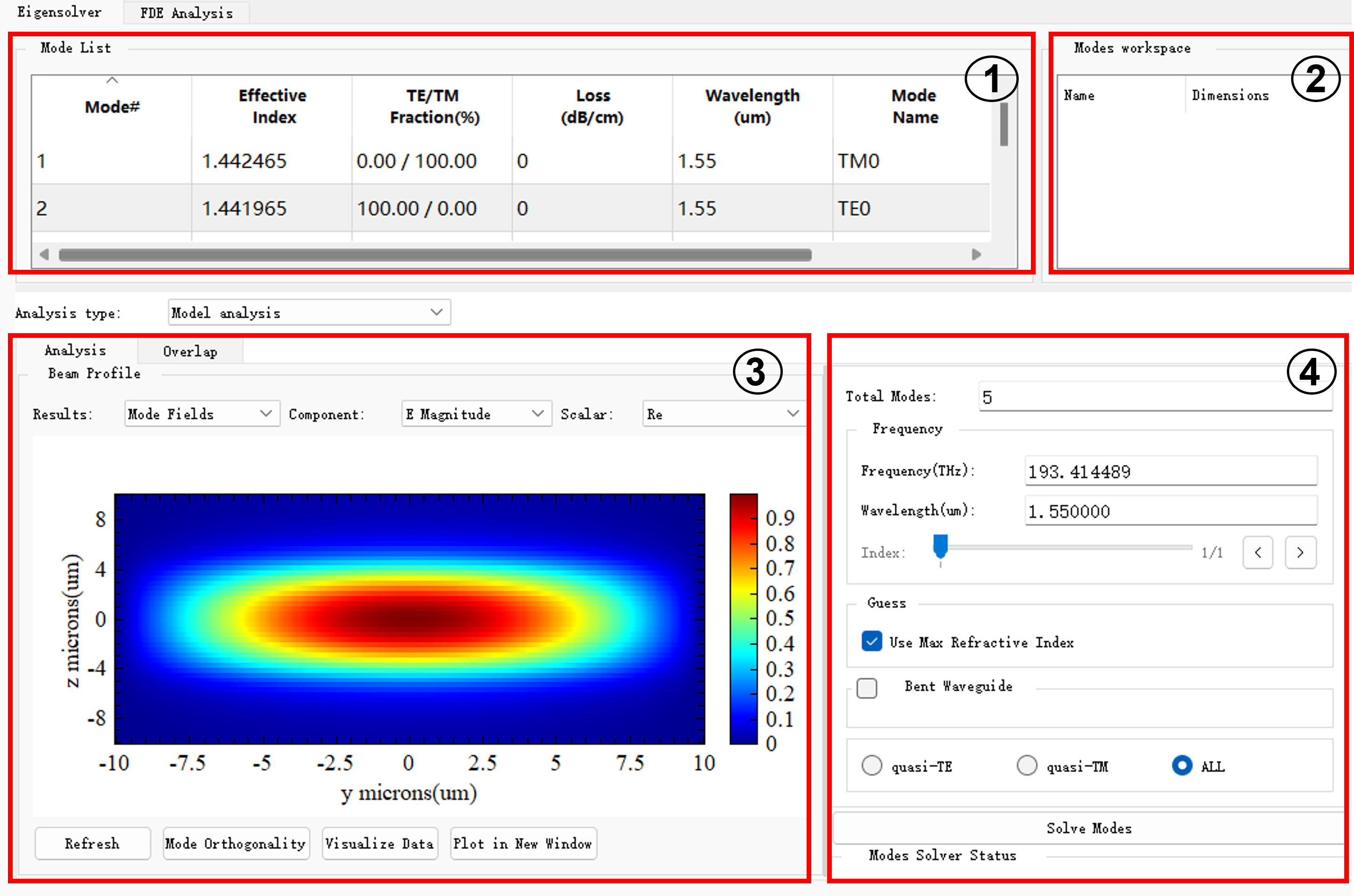
FDE仿真控制平台默认窗口如下图所示,默认窗口主要包括模式列表、模式存储、模式展示和模式分析设置四部分。
| Number | Class | Description |
|---|---|---|
| 1 | 模式列表 | 展示解模得到的模式参数。 |
| 2 | 模式工作区 | 数据存储库;存储执行复杂操作(如模态耦合)所需的所有信息。 |
| 3 | 模式展示 | 选择需要绘制的结果类型和分量等信息。 |
| 4 | 设置计算参数 | 输入模式分析所需的参数并运行解模。 |
频率分析窗口 #
分析类型(Analysis type)设置为Frequency sweep analysis时显示频率分析窗口。
频率分析窗口的界面如下图所示:

| Number | Class | Description |
|---|---|---|
| 1 | 频率分析绘图区 | 选择绘制的结果类型和分量等信息。 |
| 2 | 设置计算参数 | 自定义频率分析的参数并运行解模。 |
模式耦合窗口 #
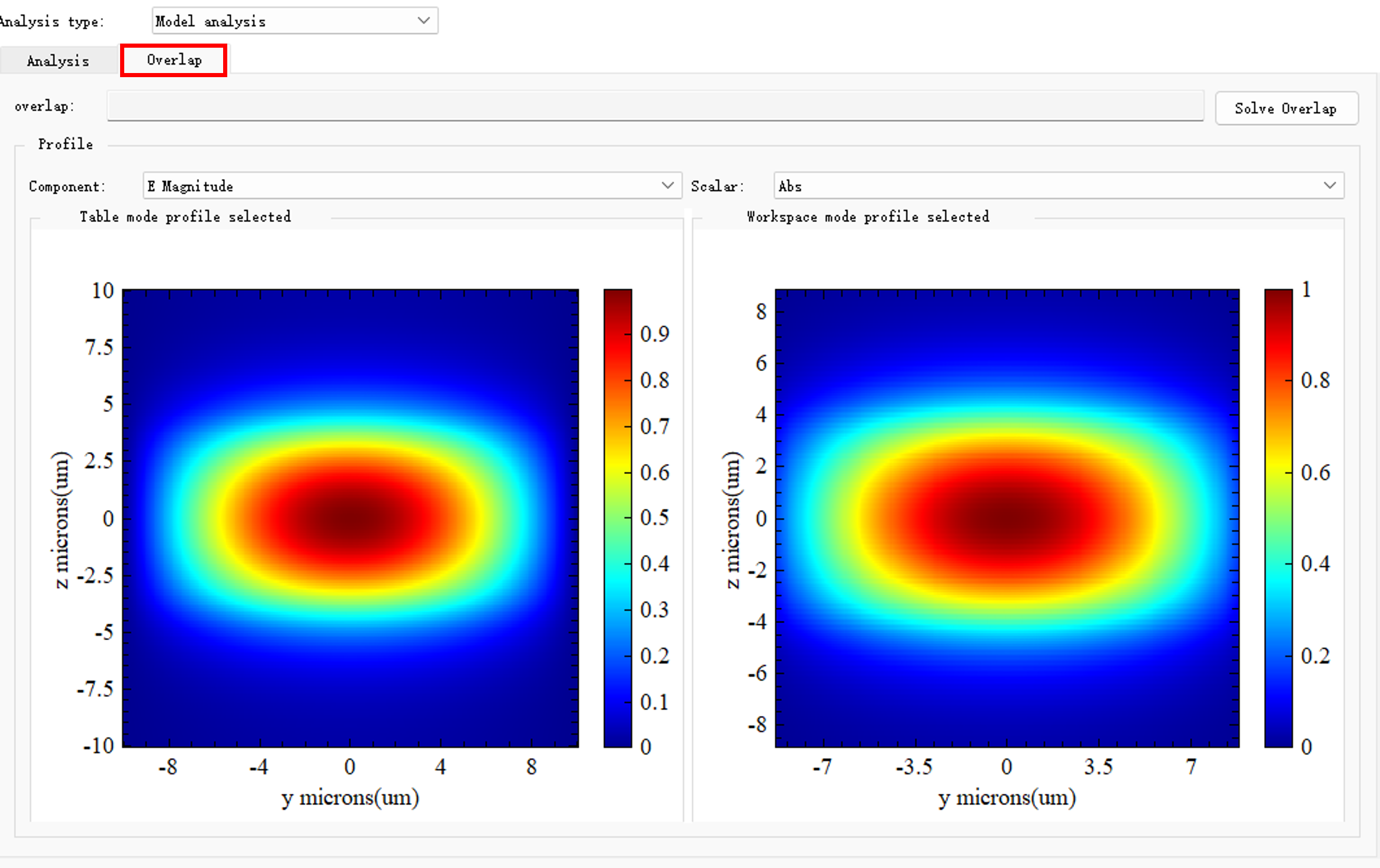
当用户切换到Overlap时,进入模式耦合界面,该界面主要显示当前选择模式的图像,以及耦合的结果数据。
FDE仿真控制平台的基本设置 #
模式列表 #
Mode list显示解模得到的模式信息。
| Name | Description |
|---|---|
| Mode# | 模式序号。 |
| Effective index | 模式的等效折射率。 |
| TE/TM fraction | 模式中TE和TM模式能量分布相对大小。 |
| Loss | 模式的传输损耗,即光信号在波导器件中由于吸收、散射等因素引起的能量衰减。 |
| Wavelength | 当前解模的波长。 |
| Mode name | 模式名称。 |
等效折射率 #
使用以下公式计算模式的等效折射率(Effective Index):
neff=vc=k0β
其中c是真空中的光速,v是模式的群速度,β是模式的传播常数,k0是自由空间的波矢量k0=λ2π。
TE/TM占比 #
TE/TM占比(TE/TM fraction(%))表示模式中TE和TM模式能量分布相对大小。其计算公式为:
TE fraction =1−∫(∣E∣2)dA∣∣∫∣E⊥∣2dA∣∣
TM fraction = 1−∫(∣H∣2)dA∣∣∫∣H⊥∣2dA∣∣
其中E⊥为沿传播方向的电场分量,H⊥沿传播方向的磁场分量,A∣∣光波导模式截面上的积分面积。
损耗 #
使用以下公式计算模式的传输损耗(Loss(dB/cm)):
Loss(dB/cm)=−0.2log10(e−2π/λ)
模式工作区 #
模式工作区(Mode workspaces)是执行复杂操作(如模态重叠)所需的所有信息的数据存储库,存储的数据可以来自模式列表(Mode list),也可以由用户导入。
下面展示将数据加载到模式工作区窗口的方法。
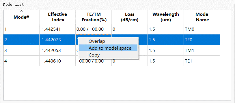
存储模式列表中的数据 #
在模式列表中通过右键单击所需的模式,然后点击Add to model space将该模式的数据加载到模式工作区。
存储用户导入的数据文件 #
在模式工作区窗口右键单击,然后点击Load选择数据文件加载到模式工作区。

| Name | Description |
|---|---|
| Name | 数据名称。 |
| Dimensions | 数据维度。 |
模式分析 #
分析类型(Analysis type)选择Model analysis为模式分析,包含设置计算参数和结果图像两部分。
光束轮廓 #
Beam profile为所选模式的数据图像。
| Name | Description |
|---|---|
| Results | 允许用户指定绘制的数据类型,下拉选择Mode fields和Index两种数据类型。 |
| Components | Results选择Mode fields时,分量可选择:E Magnitude,Ex,Ey,Ez,H Magnitude,Hx,Hy,Hz;Results选择Index时,分量可选择:Index_x,Index_y,Index_z。 |
| Scalar | Abs:所选分量的模;Re:所选分量的实数部分;Im:所选分量的虚数部分;Phase:所选分量的辐角。 |
| Refresh | 更新图像。 |
| Visualize data | 打开数据可视化窗口。 |
| Plot in new window | 将图像绘制在新的窗口。 |
设置计算参数 #
| Name | Description |
|---|---|
| Total modes | 解模的最大模数。 |
- 频率
| Name | Description |
|---|---|
| Frequency | 求解模式的频率,只读参数。 |
| Wavelength | 求解模式的波长,只读参数。 |
- 猜想
| Name | Description |
|---|---|
| Use max refractive index | 使用结构的最大折射率进行模式计算。 |
| Guess value | 指定模式计算的折射率;用于计算接近用户自定义的等效折射率值的模式,取消勾选Use max refractive index时启用该项。 |
- 弯曲波导
当求解弯曲波导的模式时启用该项。
| Name | Description |
|---|---|
| Bend radius | 弯曲波导的曲率半径。 |
| Bend waveguide width | 弯曲波导的宽度。 |
- TE/TM
| Name | Description |
|---|---|
| Quasi-TE | 准横向电场模式;Quasi-TE模式电场主要集中在垂直于传播方向(横向),在传播方向(纵向)可能存在一些非零的电场分量,而TE模式电场完全集中在垂直于传播方向(横向),即传输方向(纵向)上没有电场分量。 |
| Quasi-TM | 准横向磁场模式;Quasi-TM模式磁场主要集中在垂直于传播方向(横向),在传播方向(纵向)可能存在一些非零的磁场分量,而TM模式磁场完全集中在垂直于传播方向(横向),即传输方向(纵向)上没有磁场分量。 |
| All | 全部模式。 |
- 解模状态
| Name | Description |
|---|---|
| Solve modes | 通过点击此按钮,模式求解器将根据用户设置的参数求解模式。 |
频率分析 #
选择分析类型为 Frequency sweep analysis ,系统将自动切换到频率分析窗口。该窗口包含设置计算参数和结果图像两部分。频率分析通过在不同频率点进行模式求解,从而获得群折射率、色散和损耗等光学特性。
频率分析的计算参数设置与模式分析类似,具体配置请参考上文模式分析部分的相关说明。
跟踪指定模式 #
频率分析需在波长范围内的多个频率点进行模式求解,因此需要设置 Wavelength Point。若需对特定模式进行跟踪分析,请启用 Track Selected Mode 功能。
使用该功能的步骤如下:
- 确定要跟踪的模式。在不勾选 Track selected mode 的情况下进行频率分析,从中选定需要跟踪的模式(例如 mode#9)。
- 勾选 Track selected mode 选项,并输入波长范围。最小波长将自动设置为选定模式的波长,最大波长可以手动输入。
- 点击 Solve Modes 再次进行模式求解。

求解完成后,可在 frequencysweep 结果中查看以下内容:各个频点下所有模式的最佳模式重叠(overlap),每个频点下选定模式的模式编号(mode id),以及对应的有效折射率(neff)。同时,还保留了选定模式在各个频点下的模式场(tracked mode fields)。

模式耦合 #
当用户切换到Overlap时,进入模式耦合界面,该标签页主要用于求解模式耦合。
| Name | Description |
|---|---|
| Solve overlap | 计算模式列表的模式与模式工作区的模式的耦合。 |
| Components | 下拉选择场分量:E Magnitude,Ex,Ey,Ez,H Magnitude,Hx,Hy,Hz。 |
| Scalar | Abs:所选分量的模;Re:所选分量的实数部分;Im:所选分量的虚数部分;Phase:所选分量的辐角。 |
| Table mode profile selected | 当前选择模式列表中的模式图像。 |
| Workspace mode profile selected | 当前选择模式工作区的模式图像。 |