如何使用“对称”和“反对称边界”减少仿真空间?如何判断自己设置的“对称”和“反对称边界”是否准确? #
问题描述 #
在设置求解器时,我希望通过设置对称和反对称边界条件来减少仿真空间,提高计算效率。但是我不确定什么情况下可以使用这些边界条件,以及如何正确地进行设置。
可能的原因 #
用户在使用对称性边界条件时,需准确理解以下两点:
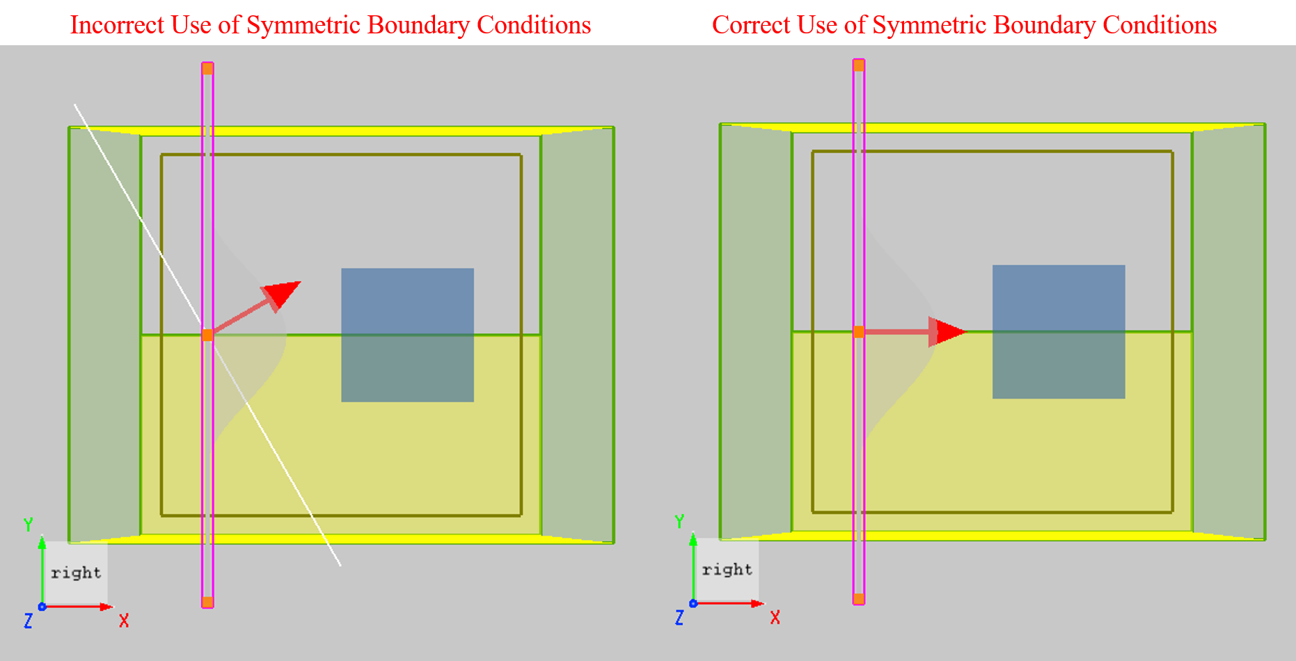
1.适用场景:对称性边界条件主要用于节省计算空间、降低内存占用并加速仿真。使用时,要求物理结构(几何与材料)对称,同时光源的场分布也需满足对称性。如下图所示,若光源为斜入射,则不满足对称性要求,无法使用对称性边界条件;而垂直入射且场分布关于对称平面对称时,则可以使用。合理利用对称性,可在每个方向上将计算区域缩减一半,从而显著提升仿真效率。
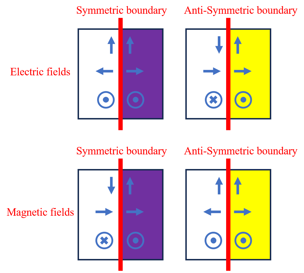
2.实现原理:对称/反对称边界条件通过在麦克斯韦方程组中,将对称平面上的特定场分量强制设为零来实现。下表列出了每种边界条件下为零的场分量。在仿真中,我们只需关注对称平面上不为零的光源场分量,即除下表所列分量之外的分量。
| 对称边界条件 | 反对称边界条件 | |
|---|---|---|
| 法向电场分量 | 0 | |
| 切向电场分量 | 0 | |
| 法向磁场分量 | 0 | |
| 切向磁场分量 | 0 |
解决方案 #
问题排查 #
在使用对称/反对称边界条件时,用户容易误选错误的边界类型。若选择错误,系统不会发出警告,但仿真结果会出现严重偏差。验证方法:可先进行一次不使用对称性边界条件的仿真,再与使用对称性边界条件的仿真结果进行对比。如果两次结果一致,说明设置正确;否则,可能存在设置错误。
解决方法 #
对称/反对称边界条件旨在提升具有对称性的仿真工程的计算效率,属于软件的高级功能。关于其正确使用方法,请参考以下要点。若仍有疑问,请联系我们。
1. 对称性边界条件需遵循一定的对称规则。电磁场在不同对称性边界条件下的分布规律如下,具体可参考对称/反对称。
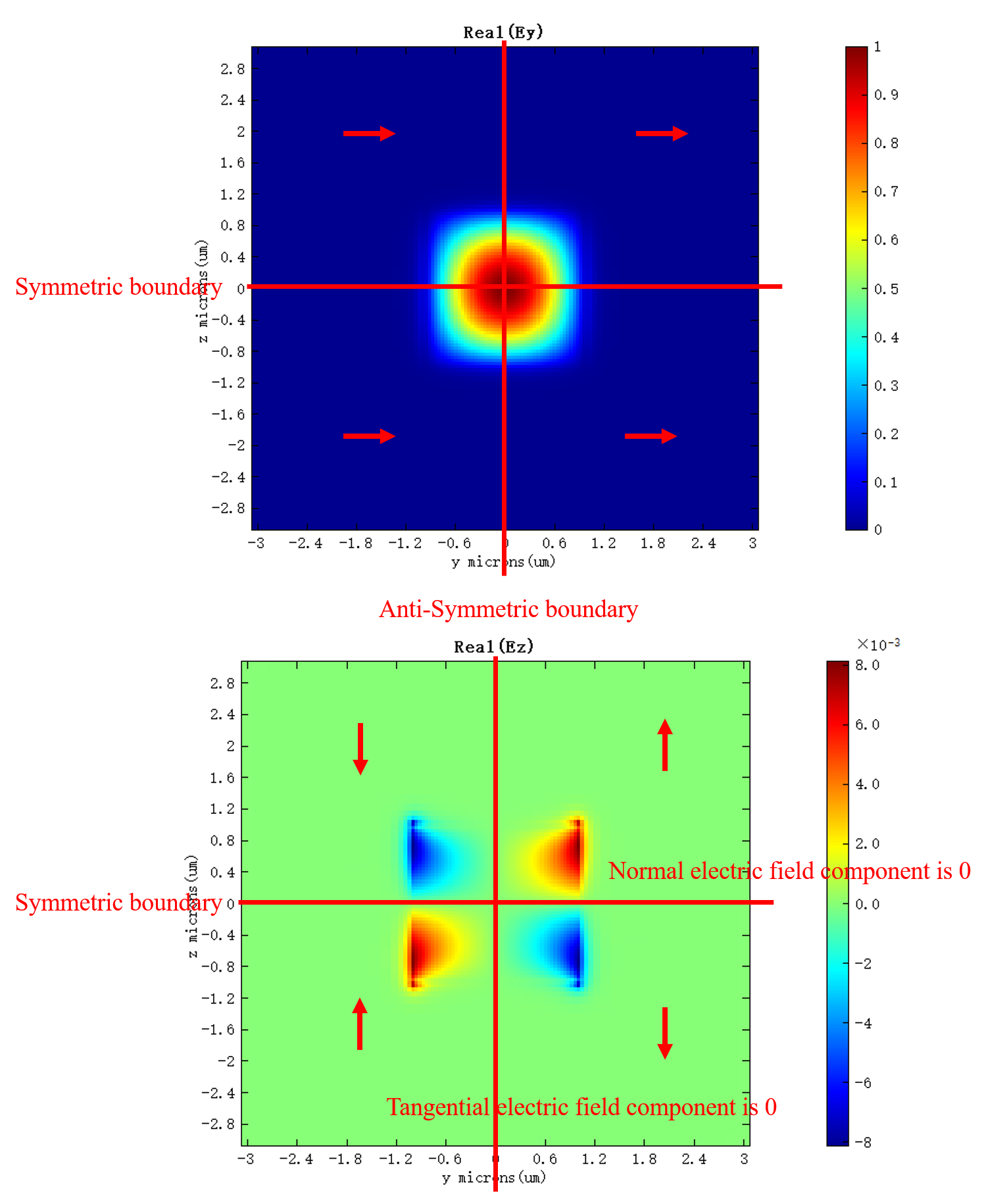
上述规则在模式源求解及腔体谐振模式研究时非常有用。如下图所示,Ey分量以向右为正方向,图中该分量在各部分均为正值;Ez分量在各部分的符号都与相邻部分相反。结合上述规则,可以确定,在Y=0处存在一个反对称平面,Z=0处存在一个对称平面。因此可将y min设置为反对称边界,z min设置为对称边界。
2. 在x/y/z方向上的min/max边界设置不同的对称性边界条件,会产生不同的效果。当某一侧边界使用对称性边界条件时,等效于采用对侧边界条件,同时节省一半的仿真空间;当同一方向两侧边界均使用对称性边界条件时,等效为周期边界条件(即空间中拥有无限个仿真周期)。
如下图所示,a、b两种设置应当等效。需要注意的是,该方向具体应采用对称边界条件还是反对称边界条件,需要根据光源的电磁场在对称平面处的分布才能确定。
- 当仿真工程使用周期边界条件,将该方向的边界替换为同类型的对称性边界,两者结果完全等效;
- 当仿真工程使用PML边界条件,将对称性方向单侧边界替换为对称性边界条件,两者结果也完全等效。
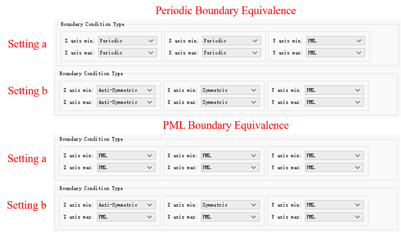
以上两种替换方法,均可将计算区域缩减至原始尺寸的1/4。需要注意:同一方向上的min/max边界,不能一边设置为对称边界条件,另一边设置为反对称边界条件。
除上述规则外,用户在使用对称性边界条件时还需注意以下事项:
- 在使用对称性边界条件后,请勿再更改仿真区域大小。此时仿真区域对应方向的一半将会以紫色或黄色阴影显示,表示该区域不会被直接仿真。
- 仿真完成后,监视器内的场数据会根据对称规则自动展开。即使实际仿真只模拟了半个区域,也能绘制整个仿真区域的电磁场分布。需要注意,部分分析组可能无法正常工作。