使用光栅投影计算任意位置的场
前言
在 FDTD 仿真中,获取器件远场分布通常有两种主流方法:一种是直接扩大仿真区域,使光传播至目标位置,这种方式虽然直观,但计算成本较高;另一种是近场-远场变换,该方法无需扩展仿真域,适用于快速估算远场行为。然而,对于周期性结构(如光栅),普通的近远场变换在处理复杂衍射级次的传播与干涉时存在局限。为此可以采用光栅投影方法,将器件近场信息分解为不同方向的平面波,进而准确重构其在均匀介质中传播至任意远场位置的结果。本案例演示了如何借助光栅投影快速计算指定远场区域的场分布,并通过与标准FDTD结果对比,验证了该方法的可靠性。
仿真设置
模型简介
本案例所用模型以玻璃为基底,其上表面覆盖一层金薄膜,金薄膜中间刻蚀有一个半径为 的孔。结构在 方向上的周期均为 。平面波光源的波长范围为 ,沿 轴正向从玻璃基底入射,电场沿 轴方向振动。根据光源和结构的对称性,在 和 方向分别使用Anti-Symmetric和Symmetric边界条件,将仿真区域缩小至原来的 。在使用对称/反对称边界模拟周期结构时,应确保对应方向的最大边界和最小边界同时设置为相应的边界类型。
仿真结果
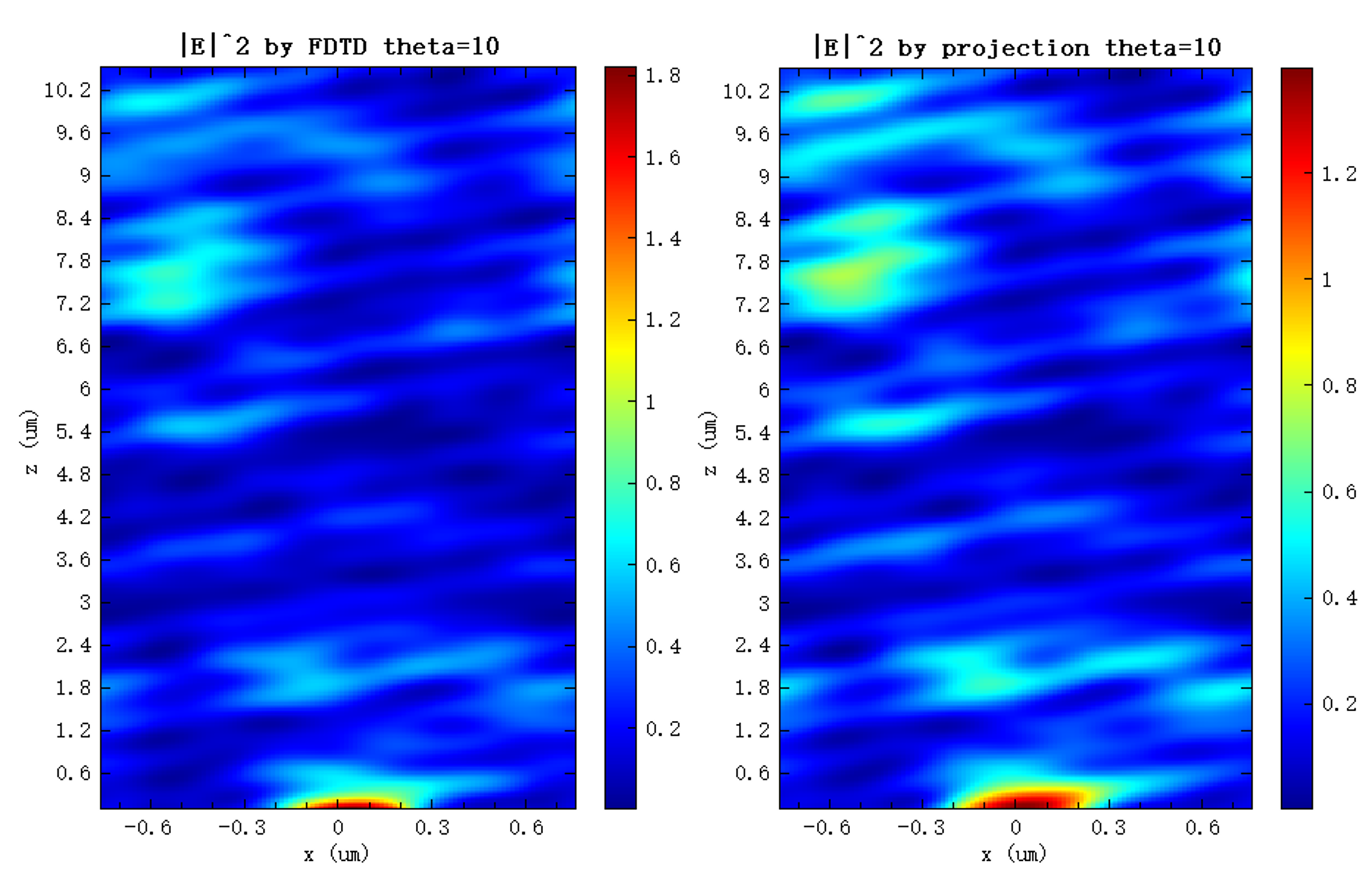
运行附件中的 solvers_propagate_periodic.msf 脚本,可以调用grating系列函数进行光栅投影,将结构上方 处 FDFP 监视器记录的电场分解为一系列平面波,然后将这些衍射平面波按照波矢关系投影到目标面,得到该位置的电场分布。下图显示了在 平面上,光传播到结构上方 处波长为 的传播电场强度分布,其中左侧为 FDFP 监视器获得的结果,右图为通过光栅投影计算得到的结果。
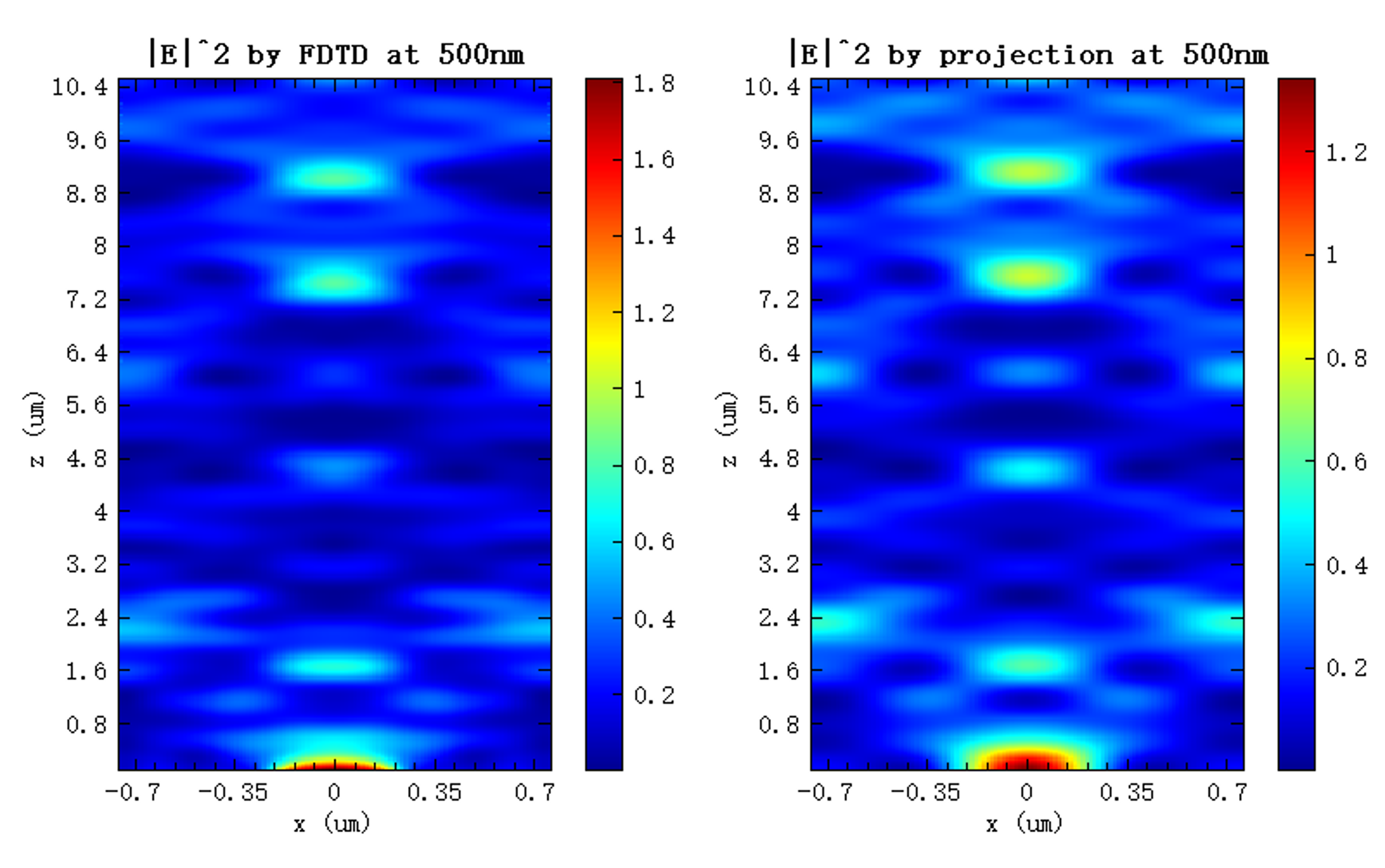
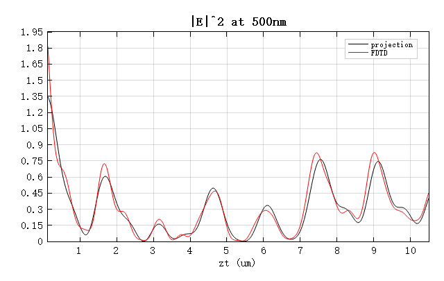
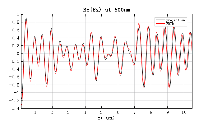
下图展示了沿 位置的电场强度以及 分量的对比结果。可以看到,投影得到的结果与 FDTD 仿真得到的结果基本一致。
值得注意的是,光栅投影法同样适用于倾斜入射的情况。下图展示了在入射角为 时,利用该方法得到的电场分布。需要注意的是,在进行倾斜入射仿真时,应将 和 方向的边界条件设置为 bloch。
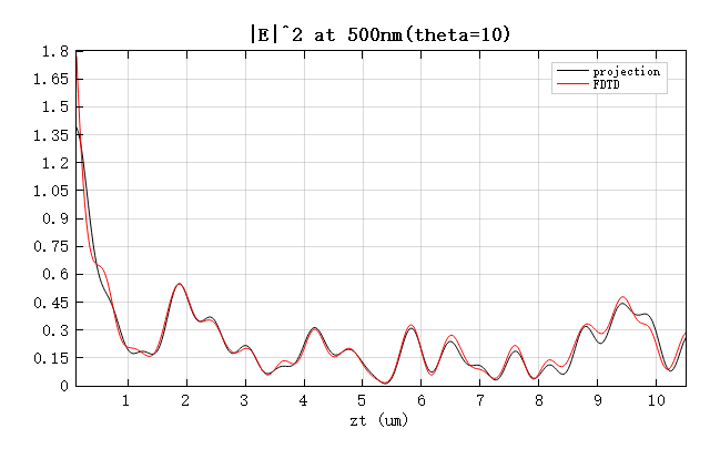
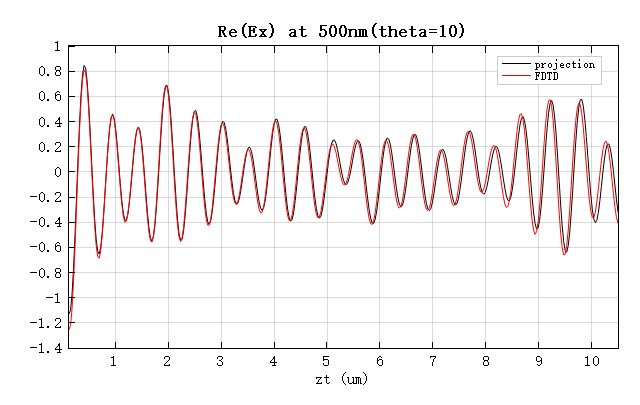
从图中可以看出,即使在倾斜入射情况下,投影计算的结果仍与 FDTD 仿真吻合。但随着传播距离增加,两者之间的差异逐渐增大,这是由于 FDTD 仿真存在网格色散效应:网格上的光速与自由空间存在微小差异,并呈现各向异性。因此,对于长距离传播而言,投影结果实际上更加精确。
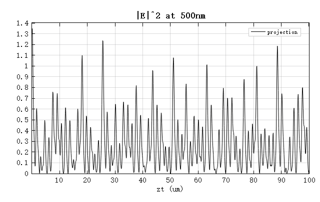
下图展示了使用投影法得到的波长为 光场,传播距离达到 。您可以将 solvers_propagate_periodic.msf 脚本中的 test 设置为0,并重新运行脚本以获得该结果。
附录
光栅投影
光栅投影是一种基于角谱理论和弗洛奎特-布洛赫定理的高效数值方法,专门用于处理周期性结构的光场传播问题。该方法将监视器中记录的近场分布按照光栅方程分解为一系列离散的衍射平面波,通过计算这些平面波在均匀介质中的传播,可以准确重构出任意指定位置处的场分布。
基本原理
对于二维周期性结构,其衍射波矢满足光栅方程:
其中 和 分别是第 级衍射光相关的面内波矢, 和 分别为 和 方向上的周期。 和 为入射波矢分量。
在已知近场分布 的情况下,可将其分解为一系列平面波的叠加:
其中系数 系数表示第 级衍射平面的复振幅,可通过 gratingvector 函数计算获得。
任意位置场分布计算
在均匀介质中,这些平面波传播到任意位置 的场分布可通过下式计算:
其中 为第 级衍射的纵向波矢分量:
这里 为自由空间波数。对于传播模式(实数的 ),该表达式描述相位积累;对于倏逝波(虚数的 ),则表征指数衰减。