硅基双直波导微环谐振腔
前言
集成光子学已成为光通信、传感和信号处理等领域的重要支撑技术。在众多光子器件中,环形谐振器因其结构紧凑、品质因数高以及优异的波长选择特性,被广泛应用于滤波、调制和非线性光学等场景。为了在目标波长范围内获得理想的谱响应,设计阶段必须进行精确的参数优化与性能预测。本案例设计仿真了一个中心波长为 ,自由频谱宽度(Free Spectral Range, FSR)为 的环形谐振器。
本文将首先利用 FDE 求解器计算 和 ,并据此选择合适的微环半径。随后,在已确定半径的条件下,分别采用 2.5D 以及3D 的 FDTD 求解器对该谐振器进行仿真,获得从输入端口耦合至 端口的透射谱及 值,并将结果与 3D FDTD 仿真结果进行对比,以验证设计的准确性与仿真方法的可靠性。
仿真设置
模型简介
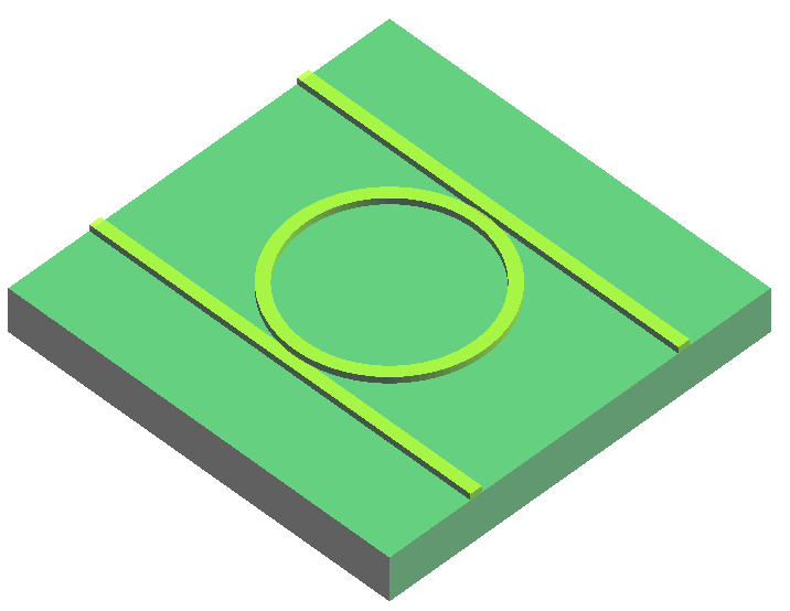
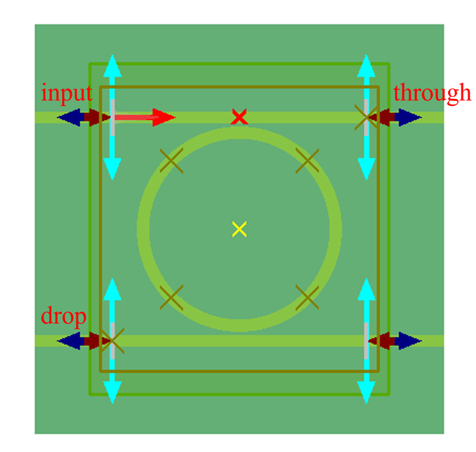
本案例采用的仿真模型如上图,波导结构为 的 SOI 波导。双直波导宽度 与微环波导宽度 相等,波导间距 设置为 。
设计要求在中心波长 处,谐振峰之间的距离(FSR)达到 (对应的波长间隔为 )。为了满足这一条件,微环半径 需要同时满足以下两个公式
其中, 、 分别为 的波长下的有效折射率与群折射率。第一个公式源于微环谐振的模式条件,保证光场在环内传播一周后相位满足相干条件;第二个公式来源于 FSR 与环长的关系,确保谐振峰间距满足设计要求。
求解器设置
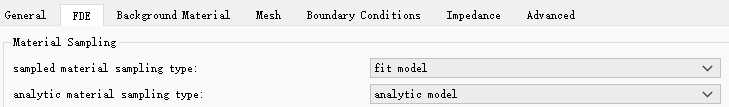
由于硅材料在光学波段为色散介质,为保证材料模型在频率范围内的连续性,需要在FDE求解器中将sampled material data sampling type设置为使用多项式材料模型拟合材料数据。
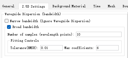
环形谐振器是一种高 Q 值的器件,为了得到更准确的仿真结果,需要较长的仿真时间,本案例中需要将 FDTD 仿真时间设置为 5 ps。在 2.5D FDTD 仿真中,由于入射光源带宽为 ,且需考虑波导色散,应在2.5D setting选项卡中勾选Broad bandwidth。此外,slab position应当选择波导所在的位置,具体可参考2.5D 求解器中的说明。
仿真结果
有效折射率与群折射率
打开附件中的 RingResonator_FDE.mpps 工程,运行 neff_ng.msf 脚本可自动设置 FDE 求解器进行模式求解与频率扫描,得到 波长下的有效折射率和群折射率:
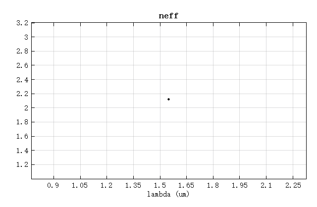
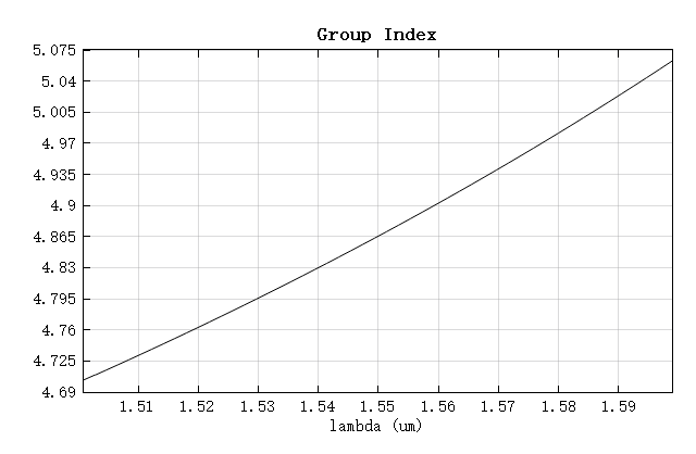
计算结果表明,有效折射率 ,群折射率 。当 时,两公式计算的半径最为接近,此时圆环半径约为 。
各端口透射谱
在 2.5D 和 3D 仿真前,均需要使用 RingResonator_structure.msf 脚本对圆环半径及端口位置等参数进行设置。下面分别给出两种仿真方法下的透射谱结果。
首先,运行 RingResonator_2.5d.mpps 工程,仿真完成后,通过 RingResonator.msf 脚本可在获得四个端口中波长与透射率的关系:
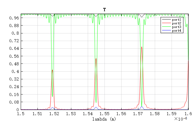
结果显示,存在三个明显的谐振峰,其中中心波长为 ,与设计值相差不到1%。该结果验证了 2.5D FDTD 在快速建模和分析中的有效性。
随后,运行 RingResonator_3d.mpps 工程,得到的透射谱如下图所示:
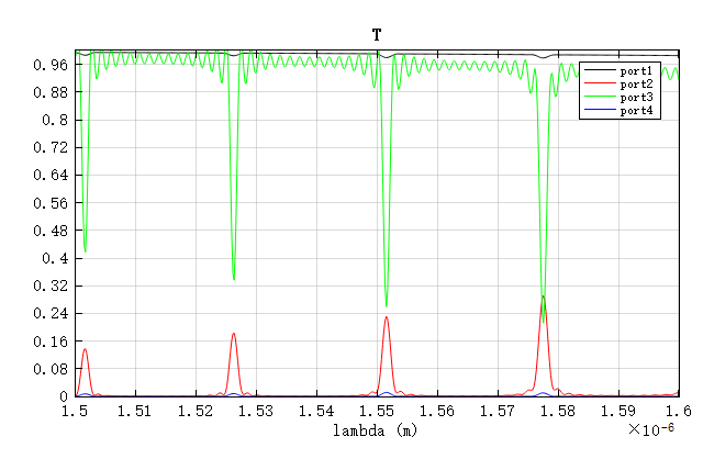
可以看到,3D 仿真得到的中心波长为 ,相比 2.5D 仿真结果更接近设计值,说明 3D FDTD 在准确性上具有优势。下文中的结果分析均为3D仿真结果。
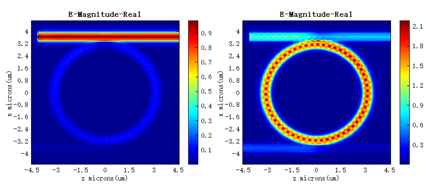
共振波长下的电场分布
根据输出端口的共振峰,查看 FDFP monitor ZX 的数据。共振峰处的电场强度如下图右所示。很明显,相对于非共振波长 (下图左),场值明显增强。
品质因子
利用工程中的 High Q analysis分析组,可得到三个谐振峰的品质因子(Q) 值:
[High Q analysis::analysis script result]
val =
Resonance 1:
val =
    frequency = 193.219THz, or 1551.57 nm
val =
    Q = 2471 +/- 0.0192705
val =
Resonance 2:
val =
    frequency = 196.43THz, or 1526.21 nm
val =
    Q = 3257.29 +/- 0.000534521
val =
Resonance 3:
val =
    frequency = 190.071THz, or 1577.27 nm
val =
    Q = 1815.94 +/- 0.127365
与理论结果对比
使用附件中的 RingResonator.msf 脚本计算出中心波长 , 时, 端口的理论频谱并与仿真结果进行对比,如下图所示。
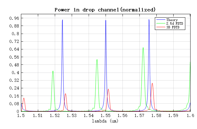
对比结果表明,FSR 与理论值吻合良好;3D FDTD 仿真得到的总透射率较低,主要由于三维仿真中引入了更多损耗因素。共振峰的精确位置对环形谐振器的有效光学长度极为敏感。两种仿真方法使用的结构相同,但在 2.5D 仿真中需要将 3D 材料等效为 2D 材料,这一过程会引入一定的近似误差,导致有效光学长度与 3D 仿真略有差异,因此峰的位置会出现轻微偏移。
参考文献
[1] Mirza, Asif , et al. "Silicon Photonic Microring Resonators: Design Optimization Under Fabrication Non-Uniformity." Design, Automation and Test in Europe Conference and Exhibition 2020.
[2] 周治平. 硅基光电子学. 北京大学出版社, 2012.
[3] Hammer, Manfred , K. R. Hiremath , and R. Stoffer . "Analytical Approaches to the Description of Optical Microresonator Devices." Aip Conference Proceedings (2004).